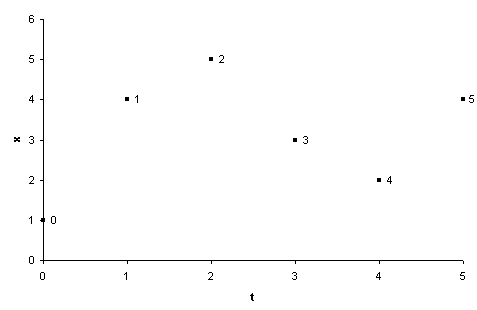
Figure 5.1 - Positions of Knots
As shown in the last example, the main problem with Bezier curves is their lack of local control. Simply increasing the number of control points adds little local control to the curve. This is due to the nature of the bleanding used for Bezier curves. They combine all the points to create the curve. The obvious solution is to combine only those points nearest to the current parameter. For this we define our points to lie in parametric space at equal intervals:
Figure 5.1 - Positions of Knots
These points are labelled internally from 0 to (number of points)-1. To calculate the curve at any parameter t we place a gaussian curve over the parameter space. This curve is actually an approximation of a gaussian; it does not extend to infinity at each end, just to +/- 2 by using the following equations:
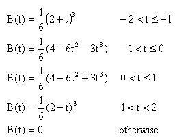
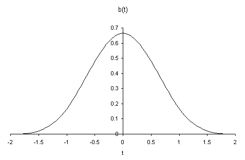
Figure 5.2 -
The Approximate Gaussian Curve
This curve peaks at a value of 2/3, and at +/- 1 its value is 1/6. When this curve is placed over the array of control points, it gives the weighting of each point. As the curve is drawn, each point will in turn become the heaviest weighted, therefore we gain more local control. The diagram below shows this curve in action. During the animation, the weighting is shown by both the size of the marker and the darkness of the line joining the marker to the curve.
Figure 5.3 - A Free B-Spline (interactive)
Notice how the curve seems to go haywire at either end. At P0, the Gaussian curve covers points from -1 to 1 (at points -2 and 2 the Gaussian weight is zero). The point at -1 is not defined, so the curve has an undefined value. In this example it is being pulled towards the origin. This behaviour is not really acceptable. One way to correct this behaviour is to duplicate the end points; if you place two points on the above diagram on top of each other, you can see how the curve comes that much closer. This is still not perfect.
What we want to do is have the curve end at the end knots. If we create the knot at -1 and just past the other end of the curve, we can do this. These made-up knots are called phantom knots. By looking at the gaussian shape, it is easy to see that when the curve is at knot 0, it takes 2/3 weight from point 0 and 1/6 from both point 1 and -1. For the point to be at knot 0, the two points at 1 and -1 must cancel each other out; that is, they must be opposite each other on the graph. You can see this in the next diagram; as you move point 0, the phantom knot always stays opposite knot 1.
Figure 5.4 - A B-Spline with Clamped Ends (interactive)
There's one other useful thing we can do with b-splines. We can make the spline go through all the knots. To do this, we define a set of parametric knots to be those required to make a b-spline go through our geometric knots. For N+1 geometric knots (those we define) there will need to be N+3 parametric knots to create the curve. This gives us two degrees of freedom; these are the gradients at knot 0 and knot N. These two sets of knots are related by equations based on the gaussian curve; for example
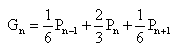
where P are the geometric knots and A are the parametric knots. The whole set of equations can be made into the following matrix equation:
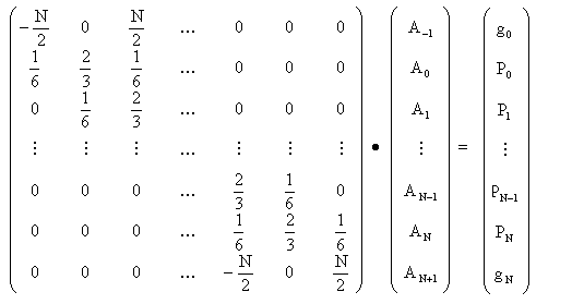
Figure 5.5 - An Interpolating B-Spline (interactive)
That completes the two dimensional segment of this tutorial. We now move on to consider how these methods are extended to defining curved surfaces.