Lecture 16: Motion and Optical Flow

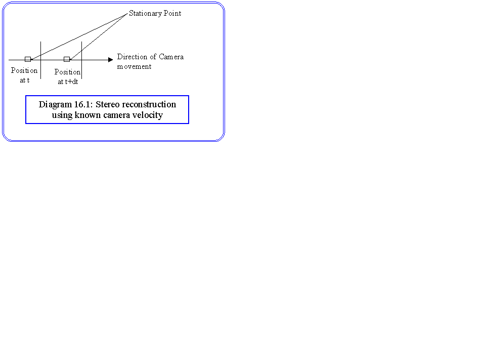
Motion adds a further dimension to computer vision, namely time. In the simplest case we can use information about the movement of a camera relative to a stationary scene in the same way that we can use multiple camera position in computational stereo (diagram 16.1). However, in most cases we will not have full information about the velocities of either the camera or the objects of the scene, and it may be these quantities that we wish to extract. The law of common fate defined by the Gestalt psychologists is applicable, ie that stimulus points moving with a common velocity can be grouped together.

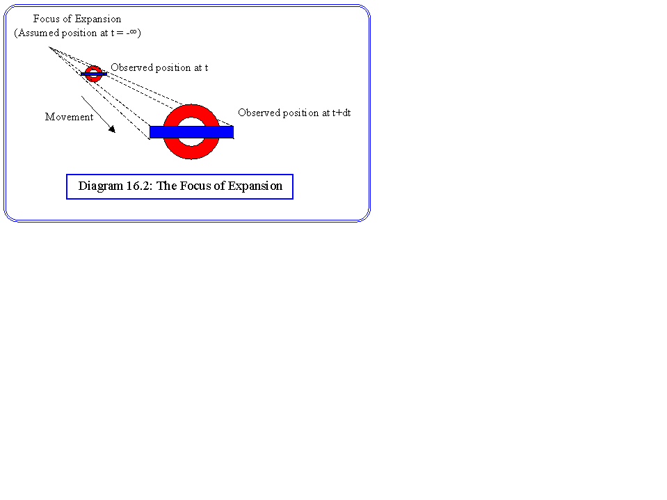
The focus of expansion.

Let us start with the simple case of a single object moving through a fixed background, with a fixed camera position. We can define a focus of expansion for that object. It is the single point on the projected image where the object appears to be comming from. First of all we define:

u = Dx/Dt, v = Dy/Dt, w = Dz/Dt

the velocity components of the moving object, and

x' = f * x/z and y' = f * y/z

the perspective projection of a point in the scene onto the camera's image plane. For simplicity we can choose our scaling so that the focal length f=1.

Consider a point at [xi,yi,zi], moving with constant velocity in the three dimensional space. Then at some time interval t later the point will have moved to:

x' = (xi + u*t)/(zi+w*t) and y' = (yi + v*t)/(zi+w*t)

to find the point where the motion apparently comes from we let t® ¥ , which allows us to eliminate [xi,yi,zi] to get:

x' = u/w and y' = v/w

This is the focus of expansion. It is a fixed point for movement with constant velocity, and is illustrated in diagram 16.2.

Time to adjacency equation

Another useful equation is the time to adjacency ratio. Suppose that we measure the distance, in the image from the focus of expansion to a moving image point, and call it D(t). If the velocity in the image is written as V(t), we have that:

D(t)/V(t) = z(t)/w(t)

Clearly, the right hand side evaluates to the time at which the moving point will cross the image plane, since w is the velocity towards the image plane, and z is the distance from it. The equation allows computation of the relative depths of two points on a moving object.:

(D1(t)*V2(t))/(V1(t)*D2(t)) = (z1(t)*w2(t))/(w1(t)*z2(t))

and since every point on the body moves with the same velocity in the 3D space:

z2(t) = z1(t) { (V1(t)*D2(t))/(D1(t)*V2(t)) }

and the x and y components can be obtained using the relations:

z(t) = w(t)*D(t)/V(t)

y(t) = y'(t)*z(t)

x(t) = x'(t)*z(t)

so, if one point is known on the body, it is possible to reconstruct the others. However, this does not result in a practical algorithm, since the ratios D(t)/V(t) cannot be measured with sufficient accuracy in a raster image.

Optical Flow

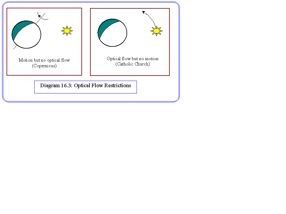
The difficulties of first of all matching points on moving objects, followed by measuring positions and velocities with sufficient accuracy, has prompted a local approach to the problem where the intensity change at one pixel is considered. Some assumptions need to be made. Diagram 16.3 shows that a rotating sphere, with fixed light and camera positions will not show any changes of pixel intensities, whereas a sphere that is stationary relative to a moving light source will display intensity changes. Similarly translation relative to a stationary light source will produce intensity changes. We assume that the lighting is stationary, and consider the movement of rigid objects relative to a fixed camera position.

Let us express the intensity at a pixel as I(x,y,t), and consider the intensity after a small change in time and position:

I(x+dx,y+dy,t+dt)

The Taylor series expansion for this is:

I(x,y,t) + (¶ I/¶ x) dx + (¶ I/¶ y) dy + (¶ I/¶ t) dt + higher order terms

Now we come to the tricky bit. Remember that we are translating an object by a small amount, [dx,dy] in the image frame. If this is sufficiently small relative to the camera and illumination, the illumination function of that point should not change, so:

I(x+dx,y+dy,t+dt) = I(x,y,t)

so, ignoring the higher order terms:

(¶ I/¶ x) dx + (¶ I/¶ y) dy + (¶ I/¶ t) dt = 0

and using the previous notation for velocity we have that:

u=dx/dt and v=dy/dt

so

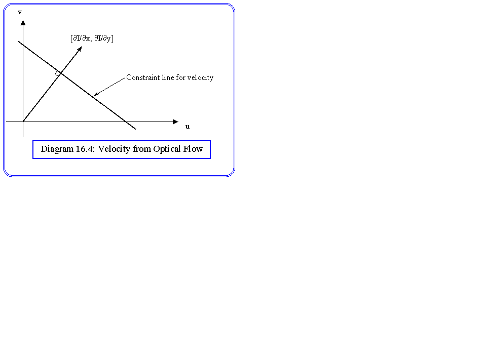
(¶ I/¶ x) u + (¶ I/¶ y) v + (¶ I/¶ t) = 0

it is possible to measure the three partial derivatives directly from the image changes at each pixel in the image. This equation is a constraint equation, which constrains the velocities to lie on a line in the u v space, as shown in diagram 16.4. The absolute values must be found by a search (relaxation) technique, which is very similar to that used in the previous lecture. For example, if we assume that we have a measure of the velocity at each pixel (ui,vi), then we can estimate the square of the error at each pixel using:

R(pi) = { (¶ I/¶ x) ui + (¶ I/¶ y) vi + (¶ I/¶ t) }²

We can also include a term related to smoothness at the pixel pi using:

S(pi) = { (¶ u/¶ x)² + (¶ u/¶ y)² + (¶ v/¶ x)² + (¶ v/¶ y)² }

These two terms combine into one error equation with the usual fiddle factor l:

E²(pi) = R(pi) + l S(pi)

We can get a global error by integrating (summing) over every pixel in the image. As before, we want to differentiate the error equation, with respect to u and v, and set the result to zero, thereby minimising the error. Again, the technique called the calculus of variations is employed. The result only is quoted:

ui = uav - (¶ I/¶ x) Q

vi = vav - (¶ I/¶ y) Q

where

Q = { (¶ I/¶ x) uav + (¶ I/¶ y)vav + (¶ I/¶ t) } / { l² + (¶ I/¶ x)² + (¶ I/¶ y)² }

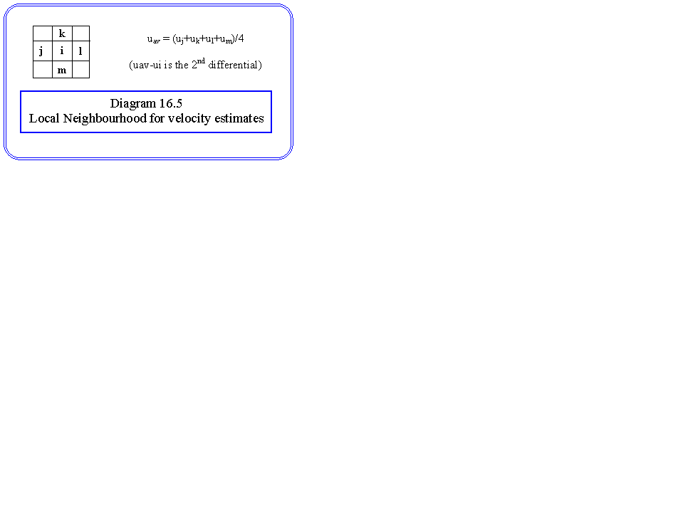
and uav and vav are the average velocities of the pixels that neighbour the one being calculated, as shown in diagram 16.5.

The relaxation iteration takes place over every pixel in the image until a stable solution is found. An alternative to iterating over the estimates based on two frames is to use a sequence of frames:

u(x,y,t) = uav(x,y,t-1) - (¶ I/¶ x) Q

v(x,y,t) = vav(x,y,t-1) - (¶ I/¶ y) Q