Trace Visualisation

The lite version ³ of the abduction (system) module can export query traces to external files in the .graphml format, which can then be visualised with the free and powerful yED Graph Editor ⁴. To generate traces for queries, a user can use the predicates eval_all_with_trace(+Query), query_all_with_trace(+Query), eval_all_with_trace(+Query, +OutputFile) and query_all_with_trace(+Query, +OutputFile). Unless an output file for the trace data is specified (i.e., using the last two predicates), the trace data is dumped to a file named trace.graphml (i.e., using the first two predicates).

Let us take the circuit diagnosis problem ⁵ as an example to illustrate the usage of this trace visualisation facility. First, download all the relevant files and load the abductive theory into the system, and then execute one of the trace predicates, e.g. (Note that the computation may take longer than that of the predicates that do not collect trace data),

| ?- load_theory('circuits-diagnosis-2.pl').
yes
| ?- query_all_with_trace([output(g2, on)]).

+++++++++++++++ Start +++++++++++++++++

Query: [output(g2,on)].
 <= [].
 <= [broken(g2),broken(g1)].

Total execution time (seconds): 1
Total explanations found: 2

---------------  End  -----------------

yes

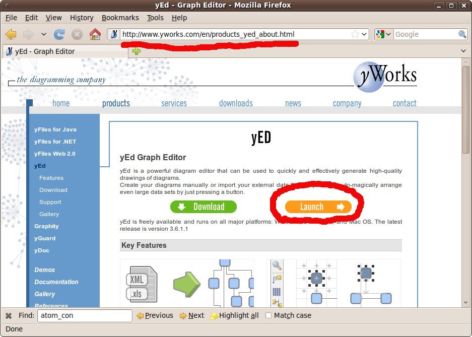
Now, there should be a file called trace.graphml in the same directory where the downloaded source files are stored. Next, we will open this file with the yED editor. The yED editor can either be downloaded from the website and run as a standalone Java application, or be launched from the website directly without installation (See Figure 1).

Figure 1: Launching yED Graph Editor

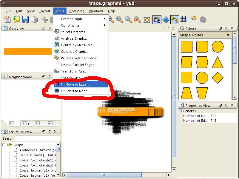
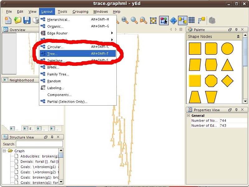
Once yED is up and running, we load the file trace.graphml. However, at this moment the file contains only raw data of the query trace, and the initial visualisation is not readable at all. We need to use several features of the yED editor to improve it. This is done through the following three steps:

1. Select Tools, then Fit Node to Label..;
2. Select Tools, then Fit Label to Node.. (See Figure 2);
3. Select Layout, then Tree (See Figure 3).

Figure 2: Resizing the Nodes

Figure 3: Layout the Trace as a Tree

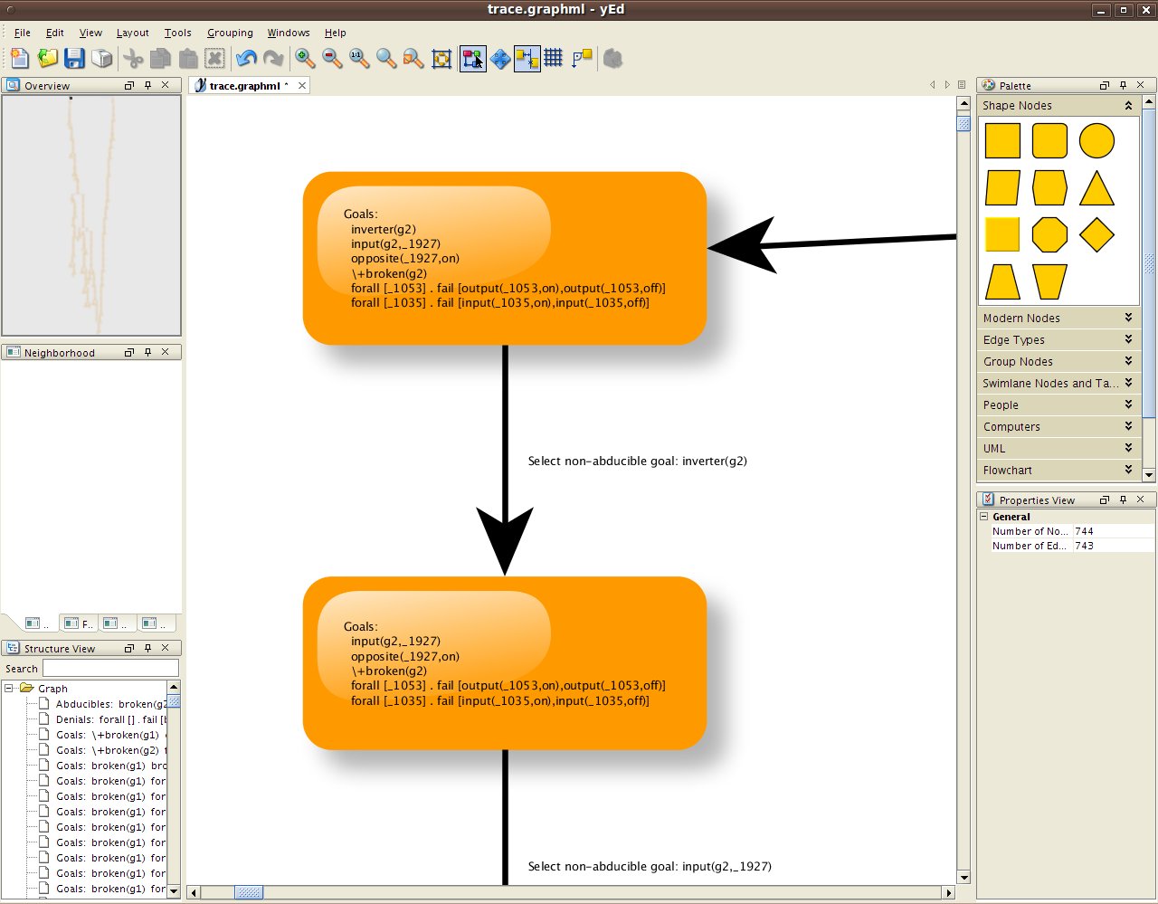
After these simple steps, the query trace is visualised as a tree, where each node represents a state containing intermediate computational data such as remaining goals, collected abducibles and collected constraints, and each edge shows the goal selected for reduction during an abductive inference step. The users can then zoom out/in to inspect the trace (see Figure 4), or even change the appearance and layout of it.

Figure 4: Inspecting the Trace