
Deductive inference derives consequences E from a prior theory T. Similarly, inductive inference derives a general belief T from specific beliefs E. In both deduction and induction T and E must be consistent and

Within ILP it is usual to separate the above elements into examples (E), background knowledge (B), and hypothesis (H). These have the relationship

B, H and E are each logic programs. E usually consists of ground unit clauses of a single target predicate. E can be separated into positive examples (E+), as ground unit definite clauses and negative examples (E-), ground unit headless Horn clauses. However, the separation into B, H and E is a matter of convenience
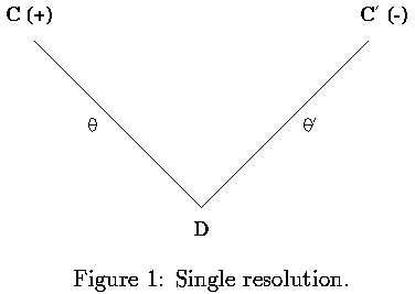
A single resolution step is shown below

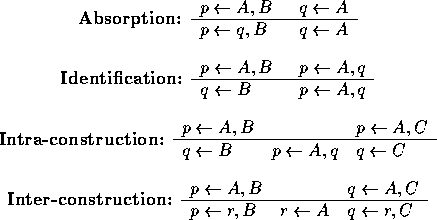
Inductive inference based on inverting resolution in propositional logic was the basis of the inductive inference rules within the Duce system.

Duce's inference rules invert single-depth applications of resolution. Using the rules a set of resolution-based trees for deriving the examples can be constructed backwards from their roots. The set of leaves of the trees represent a theory from which the examples can be derived. In the process new proposition symbols, not found in the examples, can be ''invented'' by the intra- and inter-construction rules.

Figure 1 shows a resolution step. During a deductive resolution step D is derived at the base of the 'V' given the clauses on the arms. In contrast, a 'V' inductive inference step derives one of the clauses on the arm of the `V' given the clause on the other arm and the clause at the base. In Figure 1 the literal resolved is positive (+) in C and negative (-) in C'. Duce's absorption rule constructs C' from C and D, while the identification rule derives C from C' and D.
Since algebraic inversion of resolution has a complex non-deterministic solution only a restricted form of absorption was implemented in Cigol (logiC backwards). However, there is a unique most-specific solution for `V' inductive inference rules. That is

where  is such that
  Rather than inverting the equations of resolution we might consider resolution
from the model-theoretic point of view. That is

Applying the deduction theorem gives a deductive solution for absorption.

This is a special case of inverting implication.
In the late 1960s Reynolds and Plotkin investigated the problem of finding least general generalisations (lggs) of atoms. The work focused on the importance of Robinson's unification to deduction, and searched for an analogue useful in induction. Lggs were found to be, in some sense, an inverse to unification.
Plotkin extended the investigation to clauses. He then went on to define the lgg of two clauses relative to clausal background knowledge B.
Assume that one is attempting to learn target concept T, from examples E={x_1,x_2,...,x_m}. Given background knowledge , H=rlgg_B (E) will be the hypothesis within the relative subsumption lattice with the fewest possible errors of commission (instances x in X for which H entails x and T does not entail x).
This approach to learning from positive data has the following problems.
 -subsumption
is used in place of clause implication in both. Plotkin noted that if clause
C
  -subsumes clause D (or
  )
then C -> D. However, he also notes that C -> D does not imply
  .
Although efficient methods are known for enumerating every clause C which
  -subsumes
an arbitrary clause D, this is not the case for clauses C which imply D.
This is known as the problem of inverting implication between clauses.
Gottlob proved a number of properties concerning implication between
clauses. He demonstrated that for any two non-tautological clauses, C,D,
where C+, C-, and D+, D- be the sets of positive and negative literals
of clauses C and D respectively, then C -> D implies that C+  -subsumes
D+ and C-
  -subsumes D-.
Sub-unification has been applied In an attempt to solve the inverting implication problem. Sub-unification is a process of matching sub-terms in D to produce C. It has been demonstrated that sub-unification is able to construct recursive clauses from fewer examples than would be required by ILP systems such as Golem and FOIL.
Another notable Lemma was proved by Lee. This states that a clause
T implies clause C if and only if there exists a clause D in the resolution
closure of T, such that  -subsumes
C.
In particular it is shown that Lee's subsumption lemma has the following corollary. (Implication and recursion)
Let C, D be clauses. C -> D if and only if either D is a tautology
or C  -subsumes D or there is a clause
E such that E
  -subsumes D where
E is constructed by repeatedly self-resolving C.
Thus the difference between  -subsumption
and implication between clauses C and D is only pertinent when C can self-resolve.
Attempts were made to a) extend inverse resolution and b) use a mixture
of inverse resolution and lgg to solve the problem. The extended inverse
resolution method suffers from problems of non-determinacy. Idestam-Almquist's
use of lgg suffers from the standard problem of intractably large clauses.
Both approaches are incomplete for inverting implication, though Idestam-Almquist's
technique is complete for a restricted form of entailment called T-implication.
It has been shown that for certain recursive clauses D, all the clauses
C which imply D also  -subsume a
logically equivalent clause D'. Up to renaming of variables every clause
D has at most one most specific form of D' in the
  -subsumption
lattice. D' is called the self-saturation of D. However, there exist definite
clauses which have no finite self-saturation.

Note, in general B, H and E could be arbitrary logic programs. Each clause in the simplest H should explain at least one example, since otherwise there is a simpler H' which will do. Consider then the case of H and E each being single Horn clauses. This can now be seen as a generalised form of absorption and rearranged similarly to give

Since H and E are each single clauses, their negation will be logic
programs consisting only of ground skolemised unit clauses. Let  be the (potentially infinite) conjunction of ground literals which are
true in all models of
  . Since
  must be true in every model of
  it
must contain a subset of the ground literals in
  .
Therefore

and so for all H

A subset of the solutions for H can be found by considering the clauses
which  -subsume
  .
The complete set of candidates for H can be found by considering all clauses
which
  -subsume sub-saturants of
  .
.
The major features of U-learnability that distinguishes it from PAC-learnability are:
More formally, the teacher starts by choosing distributions F and G from the family of distributions over concept descriptions H (wffs with associated bounds for time taken to test entailment) and instances X (ground wffs) respectively. The teacher uses F and G to carry out an infinite series of teaching sessions. In each session a target theory T is chosen from F. Each T is used to provide labels from (True, False) for a set of instances randomly chosen according to distribution G. The teacher labels each instance x_i in the series < x_1, .., x_m > with True if T entails x_i and False otherwise. An hypothesis H is said to explain a set of examples E whenever it both entails and is consistent with E. On the basis of the series of labelled instances < e_1, e_2, ..., e_m >, a Turing machine learner L produces a sequence of hypotheses < H_1, H_2, ... H_m > such that H_i explains { e_1, ..., e_i }. H_i must be suggested by L in expected time bounded by a fixed polynomial function of i. The teacher stops a session once the learner suggests hypothesis H_m with expected error less than e for the label of any x_m+1 chosen randomly from G. < F, G > is said to be U-learnable if and only if there exists a Turing machine learner L such that for any choice of d and e (0 < d, e =< 1) with probability at least (1-d) in any of the sessions m is less than a fixed polynomial function of 1/d and 1/e.
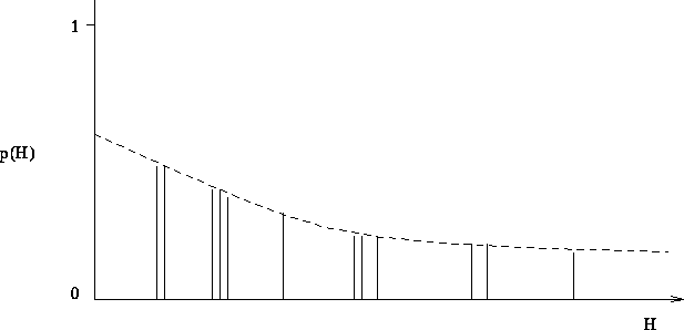
The figure below shows the effect E={e1,.., em} has on the probabilities associated with the possible hypotheses.

U-leanability may be interpreted from a Bayesian perspective. The figure shows the effect of a series of examples on the probabilites associated with hypotheses. The learner's hypothesis language is laid out along the X-axis with prior probability p(H) = F(H) for a H taken from the set of all hypotheses measured along the Y-axis, where the sum of all probabilites of the hypotheses is 1.
The descending dotted line in the Figure represents a bound on the prior probabilities of hypotheses before consideration of examples E. The hypotheses which entail and are consistent with the examples are marked as vertical bars. The prior probability of E, p(E), is simply the sum of probabilities of hypotheses in that explain the examples. The conditional probability p(E|H) is 1 in the case that H explains E and 0 otherwise. The posterior probability of H is now given by Bayes theorem as

For an hypotheses H which explains all the data, p(H|E) will increase monotonically with increasing E.
U-learnability has demonstrated positive results for the popular decision tree learning program, CART.
 Home Page