Reading Notes on Level Set Methods

Reading Notes on
Level Set Methods

Wenjia Bai

December 14, 2009

1.: Title: http://en.wikipedia.org/wiki/Geometric_flow
2.: Title: Level Set Methods in Medical Image Analysis: Segmentation
Author: Nikos Paragios
Link: http://www.wisdom.weizmann.ac.il/~boiman/reading/level_sets/levelset_tutorial.ppt

1 Geometric Flow

In mathematics, specifically differential geometry, a geometric flow is the gradient flow associated to a functional on a manifold which has a geometric interpretation, usually associated with some extrinsic or intrinsic curvature. A geometric flow is also called a geometric evolution equation. (Imagine a manifold is evolving, i.e. flowing.)

Given an elliptic operator L, the parabolic PDE u_t = Lu yields a flow, and stationary states for the flow are solutions to the elliptic PDE Lu = 0.

The elliptic PDE Lu = 0 can be associated with a functional. One can define a functional F(u) = ∫ f(x,u,u_x), which has Euler-Lagrange equation Lu = 0 for some operator L, and associated PDE u_t = Lu.

From a mathematical perspective, the level set method is a method to evolve the PDE u_t = Lu.

2 Computer Vision Perspective

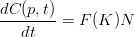
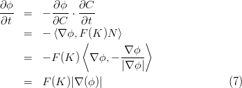
In 2-D case, the manifold is a curve C on a plane. We want to evolve the curve C so that it forms a segmentation, in other words, capturing the shape of an object or several objects. To this end, we propagate the curve using the following formula,

dC (p, t) --dt----= F (K )N

(1)

where p denotes the parameter for the curve, t denotes time, F(K) denotes speed and N denotes the normal vector, which is the direction of propagation.

So we can define some form of F(K) to drive the propagation. The curve propagation stops where F(K) = 0. A very intuitive definition is the reciprocal of the image gradient, so that curve propagation stops where the gradient is large, very likely being the boundary of an object.

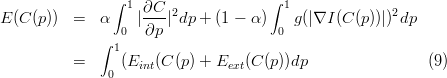
Alternatively, we can define an energy function of the form,

∫ E(ϕ ) = e(s,ϕ, ϕs)ds Ω

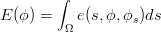(2)

where s denotes the coordinate and Ω denotes the space. Solving the Euler-Lagrange equation (Cremers’s review 2007) leads to the level set flow function,

∂ϕ ∂E ∂e ∂ ∂e ∂t-= - -∂ϕ-= - ∂ϕ-+ ∂s∂-ϕ- s

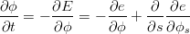(3)

3 Solution

However, if we evolve the curve C according to Eq. 1, we can never change the topology of C. The explicit representation of the curve prohibits any topological changes. The active contour snake method (Kass 1988) is such a method.

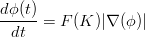
To overcome this problem, the level set method was proposed (Sethian, maybe 1988), where the curve is implicitly represented by a higher dimensional function ϕ. The curve C(p,t) is the zero level set of the function ϕ(t).

C(p,t) = {(x,y )|ϕ(x, y,t) = 0 }

(4)

ϕ(t) is a 3-D surface, whose intersection with the zero plane determines the curve C(t). When we evolve ϕ(t), the topology of C(t) can be changed.

We can write the level set formula as ϕ(C(t),t) = 0, where C(t) means a point on the curve C(t). Taking the derivative of ϕ(C(t),t) with respect to time, we have,

∂ϕ ∂C ∂ϕ ---⋅ ----+ --- = 0 ∂C ∂t ∂t

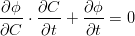(5)

We can also take the derivative of ϕ(C(t),t) along the tangential direction of the curve,

ϕ = 0 = ϕ x + ϕ y = ⟨∇ ϕ, C ⟩ s x s y x s

(6)

It leads to the conclusion that ∇ϕ is ortho-normal to C and thus the normal vector N can be represented as N = - ∇ϕ
|∇ϕ| .

It can be derived that,

∂ϕ ∂ ϕ ∂C --- = - ----⋅---- ∂t ∂C ∂t = - ⟨∇ ϕ,F (K )N ⟩ ⟨ ∇ ϕ ⟩ = - F (K ) ∇ ϕ,- ----- |∇ ϕ| = F (K )|∇ (ϕ)| (7)

It leads to the evolution function,

dϕ(t) ------= F (K )|∇ (ϕ)| dt

(8)

where ∇(ϕ) denotes the gradient of ϕ(x,y,t) w.r.t. a curve point (x,y). The Euclidean distance transform of the curve is used in most of the cases as ϕ.

The level set method can be summarised as:

1.: Determine the implicit function ϕ from the curve C using distance transform.
2.: Evolve it locally according to the level set flow Eq. 8.
3.: Determine the zero level set. i.e. the curve.
4.: Iterate till the stationary state for ϕ and C.

4 Computing Issues

4.1 Narrow Band

We are interested in the motion of the zero-level set and not in the motion of each isophote of the surface. So we only need to compute in a narrow band around the curve:

1.: Extract the current position.
2.: Define a band within a certain distance.
3.: Update the level set function.
4.: Check the new position with respect to the limits of the band.

It significantly decrease the computational complexity, in particularly when implemented efficiently. And it can account for any type of motion flows.

Another reason that I think why we should use a narrow band is that the level set flow function Eq. 8 is only valid on the curve C, as shown from the its deriving process.

4.2 Fast Marching

Central idea: move the curve one pixel in a progressive manner according to the speed function while preserving the nature of the implicit function.

I have gone through this part in Paragios’s PowerPoint but have not understood the details. Further reading is required: Tsitsiklis 1993 and Sethian 1995.

4.3 Additive Operator Splitting

Weickert introduced additive operator splitting (AOS) for fast non-linear diffusion. It accelerates the algorithm by 1 order.

5 Variations

1.

Edge-based methods

Geodesic active contours (Caselles 1997)
$∫ 1 ∂C--2 ∫ 1 2 E (C (p)) = α 0 |∂p | dp + (1 - α ) 0 g (|∇I (C (p))|) dp ∫ 1 = (Eint(C (p) + Eext(C(p))dp (9) 0$
where the E_int term controls the smoothness of the contour and the E_ext term attracts the contour towards the image features of interest. Caselles et al. gives the level set flow function after a lot of mathematical derivations.
Gradient vector flow geometric contours (Paragios 2001)
It diffuses the image gradients using gradient vector flow so that the contour can evolve even from an initial position far away from the object of interest.

2.

Region-based methods The Mumford-Shah framework (Chan-Vese 1999, Yezzi-Tsai-Willsky 1999)

∫ ∫ ∫ ∫ ∫ 2 2 E(C, μin,μout) = α Ωin(I- μin) dw+ α Ωout(I- μout) dw+ β |Cp|dp

(10)

This is a very simple model with only two classes and it assumes that the image is piece-wise constant.

3.

Hybrid methods

Geodesic active regions (Paragios-Deriche 1998)

It introduces geodesic active contours to the cost function and a Gaussian mixture model to describe the intensities of two classes. The cost function consists of both edge and region information.

4.

Multiple Phase Motion

Zhao-Chan-Merinman-Osher 1996, Samson-Aubert-Blank-Feraud 1999, and Vese-Chan 2002

The cost function consists of multiple classes in order to deal with multiple objects in an image.

5.

Knowledge-based

Leventon-Faugeras-Grimson-etal 2000, Chen-etal 2001, Tsai-Yezzi-etal 2001, and Paragios-Rousson 2002

It uses a shape model as prior in the cost function. The shape model is learnt from a training set. It turns out to be effective when there is occlusion in images.