m, where n is the number of
samples, m is the dimension, how can we find a new basis, which best
expresses the original data set?
m, where n is the number of
samples, m is the dimension, how can we find a new basis, which best
expresses the original data set?
Title: A Tutorial on Principal Component Analysis
Author: Jonathon Shlens
Given a data set X = {x1,x2,…,xn} m, where n is the number of
samples, m is the dimension, how can we find a new basis, which best
expresses the original data set?
Let P be the linear transformation matrix to the new basis, the data set expressed by the new basis is,

How do we define being a good basis?
A good basis should correspond to the directions with largest variances, because we regard that the variances contain the dynamics of interest. Also, the dynamics along different directions should be decorrelated. These directions with largest variances are called principal components.
How to mathematically describe being a good basis? After subtracting the means from each dimension of the data, we define a covariance matrix Cx,
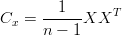 | (1) |
Cx is a m-by-m matrix. The diagonal element, the iith element, is the variance of ith element of the data. The off-diagonal element, the ijth (i≠j) element of Cx is the covariance between the ith and the jth elements of the data.
If the basis is good, then the covariance matrix Cx is diagonal, so that we can easily select the principal components according to the variances and the dynamics along different directions are decorrelated.
A symmetric matrix can be diagonalized by an orthogonal matrix of its eigenvectors. Since Cx is a symmetric matrix, it can be diagonalized,
 | (2) |
where the column vectors of P are the eigenvectors, Σ = diag(σ1,σ2,…,σm).
We can derive that,
We can then select the directions with the largest eigenvectors as the principal components.
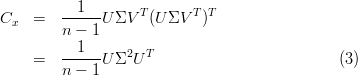
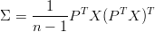
In singular value decomposition (SVD), we can decompose a m-by-n matrix X into the product of a m-by-m orthogonal matrix U, a diagonal matrix Σ, and the transpose of a n-by-n orthogonal matrix V ,

Applying SVD to Equation (1),
Compare it with Equation (2), we can see that the orthogonal matrix U is exactly P, and the diagonal matrix in Equation (3) divided by (n - 1) is equal to that in Equation (2). The new data set is Y = UT X = ΣV T .
Therefore SVD is another solution for PCA. In fact, SVD and PCA are so intimately related that the names are often interchangeable. They both reveal the structure of the matrix, or the data set, X. That is why they are abundantly used in many forms of data analysis, as a simple non-parametric method for extracting relevant information from confusing data sets.
Both the strength and weakness of PCA is that it is a non-parametric analysis. On one side, there are no parameters to estimate or adjust. The answer is data-driven, not dependent on the user. On the other side, it does not take into account any a-priori knowledge, as the parametric algorithms do.
The means of each dimension should be subtracted first, i.e. that the data set is zero means, so that Equation (1) can represent the covariance matrix.
When PCA selects the principal components, it assumes that the mean is zero and the variance of the data characterizes the dynamics of the signal. The mean and variance are statistically sufficient only for exponential distributions, e.g. Gaussian, exponential, etc.
The principal components are orthogonal. However, the orthogonal basis is not always the best description for the data set.