Lecture 3: Region features and merging criteria
In the previous lecture we looked at intensity mean and variance as the properties on which to base our segmentation algorithms. While this is a good approach for many cases, other properties are often necessary to achieve the segmentation we require. We will now look at some of these.
Colour Spaces
Colour provides an important property on which we could segment images, and it has advantages over intensity mean in certain cases. In practical systems colour is normally represented using the tri-stimulus model. Each pixel of a discrete image is specified by three bytes corresponding to the values of the red, green and blue components. Each of these could be treated as a separate image plane, and, depending on the application, we could choose to perform a segmentation on one of these planes, for example the red plane. This approach turns out to be of limited application, and a more appropriate method is to utilise a different colour space, where the same information is represented in a way that corresponds better to the segmentation method. There are many possible representations, and we will look at just one the HSI (Hue, Saturation and Intensity) space. Here again the colour image is represented in three planes which can be calculated as follows:
I = ( r + g + b )/3
S = ( max(r,g,b) - min(r,g,b) ) / max(r,g,b)
Hue (which is an angle between 0 and 360o) is best described procedurally:
if (r=g=b) Hue is undefined
if (r>b) and (g>b) Hue = 120*(g-b)/((r-b)+(g-b))
if (g>r) and (b>r) Hue = 120 + 120*(b-r)/((g-r)+(b-r))
if (r>g) and (b>g) Hue = 240 + 120*(r-g)/((r-g)+(b-g))
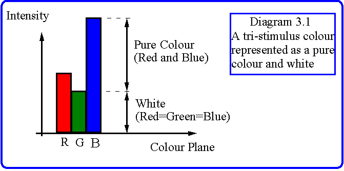
Note that every colour in the r,g,b system is made up of a white component whose magnitude is the minimum out of r g and b, and a pure colour defined by the ratio of the two non-zero colours when the white component has been subtracted. (Diagram 3.1) The saturation is the proportion of pure colour. Since hue is represented by an angle in the range 0..2p and saturation in the range 0..1 we can represent each point in r g b space on a unit circle as shown in Diagram 3.2. The centre of the circle is white (r=g=b) and the perimeter is the fully saturated pure colours. It will be seen that Hue has several immediate advantages over intensity for image segmentation. For example, objects crossed with shadows will have a constant hue and saturation at every point, but a big discontinuity in intensity. Similarly specular highlights (at least for white light) will have the same hue (though different saturation and intensity) from the rest of the object to which they belong.
Clusters and Histograms
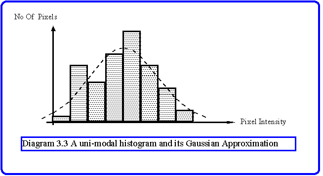
Analysis based on mean and variance makes an important assumption, namely that the feature upon which segmentation is based is distributed normally. That is, if we construct an histogram of the property it will have the shape shown in Diagram 3.3. This shape is modelled by the Gaussian distribution, G(x)= a exp(-(x-µ)2/2n) , where the peak occurs at µ (the mean) and has magnitude a. In the standard form the value of a is taken to be 1/sqrt(2pn) which ensures that the integral of the distribution is 1. For modelling histograms we should compute the area under the histogram and then divide by Sqrt(2pn) to find the correct normalisation. The parameter n is called the variance (s=sqrt(n) is the standard deviation), and measures the flatness of the distribution. Discrimination between adjacent areas with differing means and standard deviations can be made according to Fischer's criterion:
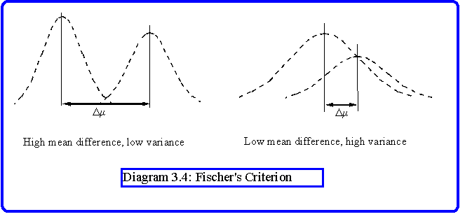
|µ1-µ2|/sqrt(n12+n22) > q
where q is a threshold. In other words, if two regions have good separation in their means, and low variance, then we can discriminate them. However, if the variance becomes high and the mean difference is low it is not possible to separate them. (Diagram 3.4)
Uniformity
For the best effect, the merging threshold for the mean intensity for two adjacent regions, q, should be adjusted depending on the expected uniformity of the merged region. Less uniform regions will require a lower threshold to prevent under merging. The uniformity is a function of both intensity mean and variance of the region. A suitable heuristic law for combining both properties into one is:
Uniformity = 1-u/m2
Note that the uniformity will be in the range 0 to 1 for cases where the samples are all positive. The threshold value, q decreases with the decrease in uniformity as follows:
q = (1 - u/m2) q0
This has the advantage that the user need only supply a single threshold, q0.
Textures and co-occurrence
In many cases, the assumption of a unimodal histogram does not hold. Areas without unimodal histograms are called textured, and require a different method of characterisation. A simple example will illustrate the difficulty. Consider an image with a region made up of small squares in a chess board pattern, alternatively black and white. In that region, the histogram consists of two peaks, one at 0 and the other at the maximum intensity, The mean will be the mid grey level, but the variance will be very high. Region growing from relatively small seeds will be impossible since all previous merging criteria will be broken.
One general method for determining the characteristics of a textured region is to use the region histogram. This can be extracted at any degree of precision, as required by the application, down to the resolution of the image. Histogram computations can be carried out recursively when building a tree, in the same manner as mean and variance were treated in the previous lecture. When comparing the histograms of two textured regions, it is necessary to normalise them to allow for different region sizes. The similarity of two regions can be measured by taking the Euclidean or Manhattan distances that separate the normalised histograms. This approach is easy to compute, but it will not separate different patterns which have the same distribution of pixel intensities. (These may be rare in practice, though they are not unheard of.)
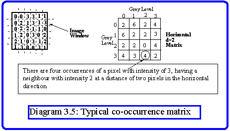
One of the ways of dealing with structure in texture is to attempt to identify repeated spatial patterns. This is done by the computation of a number of co-occurrence matrices, which essentially measure the number of times a pair of pixels at some defined separation have a given pair of intensities. A co-occurrence matrix has a size equal to the number of grey levels in the image, and is computed for a given direction and a given distance. Let us suppose that the direction is horizontal and the distance is two pixels. The row and column addresses in the matrix represent the grey levels, so for example the entry at row 3 and column 2 represents the number of times in the image that a pixel of intensity 3 has a neighbour at a distance of two pixels in the horizontal direction with intensity 2. To make the technique practical we would normally quantise the image into a small number of grey levels, typically not more than sixty four, before applying this technique. The distances could be restricted to four pixels and the directions to four (the horizontal, vertical and two diagonal directions). Thus from a texture window of any size we would extract sixteen matrices. An example of an eight by eight window with just four grey levels is given in Diagram 3.5 along with one of sixteen the co-occurrence matrices. Notice that the computation is irregular at the window boundaries, since the boundary pixels have fewer neighbours than those in the centre. This effect can be compensated by using the pixels in neighbouring regions, but for large windows it is unlikely to cause any particular problems.
Having extracted the co-occurrence matrices we are faced with the problem of how to match them. The first step that is required is to normalise them so that the entries become probabilities of co-occurrence, and are therefore independent of window size. Matching can be carried out by extracting a number characteristic properties of the matrices. For example we could compute
| Energy | S | P2(i,j) |
| i,j |
which reduces each of the normalised co-occurrence matrices to a single number. If we consider the energy of the sixteen matrices to form a characteristic vector, then the difference between two windows containing texture can be measured by either the Euclidean or the Manhattan distance between their vectors. There are many other properties, from which characteristic vectors can be derived, examples being:
| Entropy | S | - P(i,j) log2(P(i,j)) |
| i,j | ||
| Contrast | S | P2(i,j) |
| i,j | ||
| Maximum | max | P2(i,j) |
| i,j |
and so on. Co-occurrence matrices work well in specific applications, but are limited in that they cannot cope with stochastic textures, or with textures where the granularity cannot be made to match the pixel size.