Lecture 11: Fourier Methods
We have already considered some methods of classifying objects by:
1. Their two dimensional shape properties such as moments of intensity
2. The coding of a known shape for recognition by the Hough transform
3. The use of the correlation integral for direct template matching.
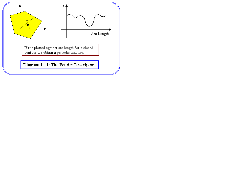
A further alternative is to classify objects by their features in the frequency domain, rather than those in the spatial domain. A simple analogy is with sound waves. A periodic sound wave can be easily described by a sinusoid of fundamental frequency, which determines the pitch, and a set of overtones, which are higher frequency sinusoids added to the fundamental which determine the timbre of the sound. All periodic functions can be broken into a set of sinusoidal waves. One simple way of associating a periodic function with an object is shown in Diagram 11.1. A fixed point, called the centre, is defined within the object by some unique means, such as averaging the boundary points. A start point on the boundary is defined again uniquely, in this case by taking the intersection of the boundary with a horizontal line through the centre. The boundary may then be described by plotting the radial distance of each boundary point from the centre against its distance along boundary from the start point. The variation of magnitude with distance along the boundary is a periodic function. If the total length around the boundary is L the period is normalised to 2p by multiplying a length l by 2p/L. If we can find the frequency components of that period function, then these can be used to classify objects in a recognition algorithm. Normally, we will choose our functions to be periodic over the interval [0..1], thus for all x, f(x)=f(x+1), and we can write:
| f(x) = a0 + a1Cos(q) + b1Sin(q) + a2Cos(2q) + b2Sin(2q) + a3Cos(3q) + b3Sin(3q) + &c |
(11.1) |
where q=2px, and ranges from 0 to 2p in the fundamental period. Gathering the terms we can write
|
¥ |
|||
| f(x) = |
S |
(ah Cos(2pxh) + bhSin(2pxh)) |
(11.2) |
|
h=0 |
where h is an integer representing the harmonic number. The Fourier transform is from the space where f(x) is represented against x, to the space where both ah and bh are represented against h. In other words it is a transform from a scalar to a vector space. It can be also be written in terms of magnitude (mh) and phase fh as
| ¥ | |||
| f(x) = | S | mh Cos(2pxh + fh) | (11.3) |
| h=0 |
To understand the transform we need first to observe some properties of orthogonal functions, in particular that:
|
2p |
|||
|
ò |
Sin(pq) Sin(qq) dq = 0 |
for integer p and q and for p¹ q |
(11.4) |
|
0 |
We can prove this by examining the expansion of Cos(q+f) from which we see that:
Sin(q)Sin(f)= (Cos(q-f) - Cos(q+f))/2
Substituting this into the integral, and assuming without loss of generality that q<p we get
|
2p |
|
|
ò |
(1/2) (Cos((p-q)q) - Cos((p+q)q) dq = 0 |
|
0 |
Which clearly integrates to zero over a whole period, except where p=q when the first term becomes a half, and the integral evaluates to p. Notice that this result is independent of p and q. There are two further results that we need which can be proved similarly:
|
2p |
||
|
ò |
Cos(pq) Cos(qq) dq = 0 | for integer p and q and for p¹ q |
|
0 |
||
|
2p |
||
|
ò |
Cos(pq) Sin(qq) dq = 0 | for integer p and q |
|
0 |
Since we are only interested in the discrete transform, which is the form in which we will compute it, we can approximate the above integrals (for example equation 11.4) by sums as follows:
|
N-1 |
||
|
S |
(1/N) Sin(2ppx/N) Sin(2pqx/N) = 0 |
for integer p and q and for p¹ q |
|
x=0 |
With similar results for Cos Cos and Sin Cos. Notice that when p=q the sum will evaluate to approximately 1/2 due to the normalising factor (1/N). Now we can demonstrate how to compute the Fourier transform in two parts, first the discrete cosine transform:
|
N-1 |
||
|
Fc(u) = (1/N) |
S |
f(x) Cos(2pux/N) |
|
x=0 |
If we consider substituting for f(x) using equation 11.2 above, we can see that we have a set of Sin*Cos terms, which all sum to zero through the orthogonality property, and a set of Cos*Cos terms, which again will sum to zero for the one except where u=h, thus:
Fc(u) = au/2
Similarly we can define the discrete sine transform
|
N-1 |
||
|
Fs(u) = (1/N) |
S |
f(x) Sin(2pux/N) |
|
x=0 |
Which for some integer u will evaluate to bu/2. The Fourier transform, as we have noted yields a vector result, of which the elements are just these two scalar transforms. The complex number notation is used to produce a combined equation:
|
N-1 |
||
|
F(u) = (1/N) |
S |
f(x) (Cos(2pux/N) + j Sin(2pux/N)) |
|
x=0 |
which is written more simply as
|
N-1 |
||
|
F(u) = (1/N) |
S |
f(x) exp(-2pjux/N) |
|
x=0 |
The inverse transform is given by
|
N-1 |
||
|
f(x) = |
S |
F(u) exp(2pjux/N) |
|
x=0 |
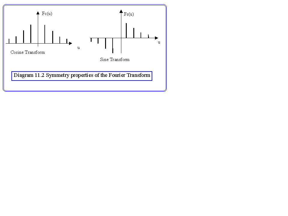
The transform can be calculated directly from the above equations, but in practice an ingenious fast Fourier algorithm, which makes use of the symmetries in the Cosine and Sine functions to reduce the number of multiplies, is used. Details of how it works can be found in any text on signal processing, and the code that implements it is widely published. Notice, that because of the symmetry properties of the sine can cosine functions the spectrum is well defined for negative values of u, as shown in Diagram 11.2. Now we return to consider how to use it in computer vision.
The advantage of using the Fourier transform is in its invariant properties. Considering the Fourier descriptor of Diagram 11.1 again, it is easy to see from equation 11.3, that rotating the object merely causes a phase change to occur, and the same phase change is caused to all the components. In the Fourier spectrum the magnitude given by: Ö (Fs(u)2 + Fc(u)2) and the phase by arctan(Fs(u)/Fc(u)). The magnitude is independent of the phase, and so unaffected by rotation. (This is an example of the very important property of shift invariance).
Secondly, consider a change of size of the object. This does not change phase, and changes all the magnitudes by the same factor. If the magnitude of the spectrum is normalised, such that its maximum is say 1, then this normalised spectrum is invariant to object size.
Lastly, consider the effect of noise and quantisation errors on the boundary. This will cause local variation of high frequency, and will not change the low frequencies. Hence, if the high frequency components of the spectrum are ignored, the rest of the spectrum is unaffected by noise.
Thus, for object recognition, the Fourier descriptor offers many advantages over the template matching methods by correlation or by Hough transform, and it is faster to compute.
Correlation and Convolution.
A theorem which should be noted is that if we have two functions, f(x) and g(x) then:
F(u) G(u) is the transform of the convolution of f and g
and F(u) G(u)* is the transform of the correlation of f and g
(G(u)* is the complex conjugate of G(u))
So, if we can compute the transforms quickly, then we can also do template matching by simply carrying out pointwise multiplies of the spectra, and taking the inverse transform. However, this technique is rarely used, since the result for continuous space does not generalise to discrete space very well.