Lecture 13: Tomographic Imaging

The name tomographic imaging is applied to scanning imagers which give images of the internal structures in the body in two dimensional slices. There are several technologies for doing this of which the most important are Computer Tomography (CT). Nuclear Magnetic Resonance (NMR) and Positron Emission Tomography (PET). We will look briefly at some of the techniques in the first two, and in particular how to use the Fourier transform to process the data.

Computer Tomography (CT)

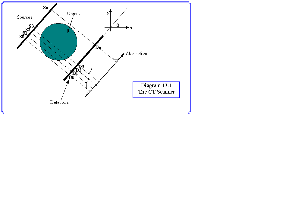
The basic principal is shown in Diagram 13.1. The internal structure being measured is projected onto the line D according to the rule that at point di, the projection takes the value of the integral along the line si to di. Thus, if we assume that the value 1 is placed inside the organ being scanned, and 0 outside, the value at di is simply the length of the line si to di which falls inside the organ. In practice, each line corresponds to an XRay emanating from the source si, being attenuated an amount proportional to the distance traveled through the organ, and then measured at the detector di. These one dimensional projections are measured for a number of values of the angle q. In the original systems, projections were taken every degree, 180 in all. The problem for the vision system is how to reconstruct the cross sectional shape from the measurements.

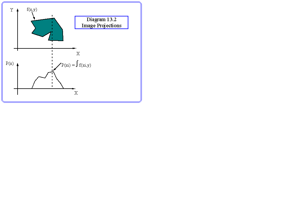
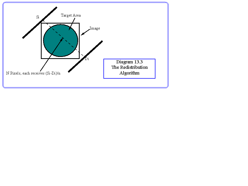
A simple algorithm which was tried originally was to simply generate a histogram of the image space. For each value of q, the value for each detector was redistributed equally among the histogram points on its line (Diagram 13.2). At the end, a threshold was applied to find the real boundary. This method was crude, and caused blurring of the boundary. A better method was devised using the FT. We first reconstruct the Fourier transform of the image of the slice, and then invert it to find the spatial picture. The way this is done used a property of the Fourier transforms of projections of an image. Consider first the projection for which q=0, that is to say, the projection onto the x axis, which in discrete form is defined as:

where f(x,y) is the image. We see the projection as the average of all the pixels on a vertical line of the image (Diagram 13.3). Now we take the one dimensional FT of the projection:

Looking back to the definition of the discrete Fourier transform

we see that

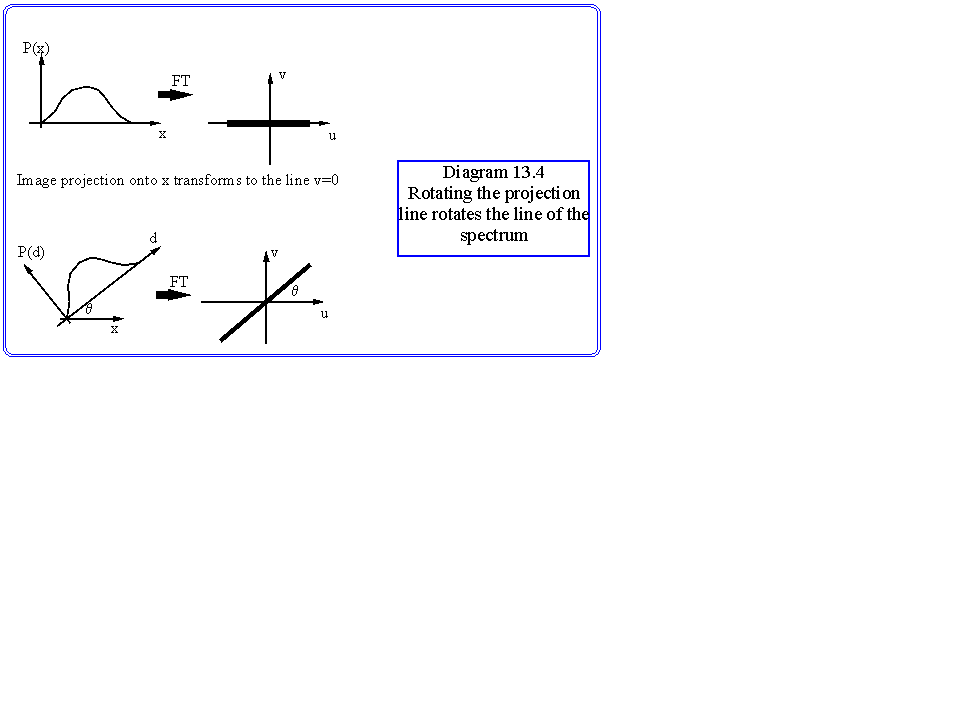
P(u) = F(u,0)

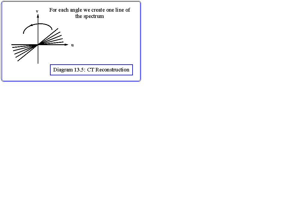
That is to say, the transform of a projection of an image onto the x axis is simply the line of the transformed image where v=0. Now we apply the important property that rotation about the origin is preserved in the FT. So, if we consider a projection where the measuring equipment has been rotated through q degrees, the transform of that projection will appear along a line at q degrees to the u axis in the FT, as shown in Diagram 13.4.

Now, each measurement we take in a CT scan is indeed a projection, because the absorbencies of the materials to the x rays add along the line from S to D. Thus for each of the measurements we compute one line of the spectrum (Diagram 13.5). When all the measurements have all been taken, we then interpolate to find the missing points in the spectrum, and take the inverse transform to reconstruct the spatial data. In practice interpolation is not a very satisfactory solution due to the discrete nature of the spectrum. Instead the inverse transform is taken using polar co-ordinates, and the transform to Cartesian co-ordinates is carried out in spatial domain.

NMR images.

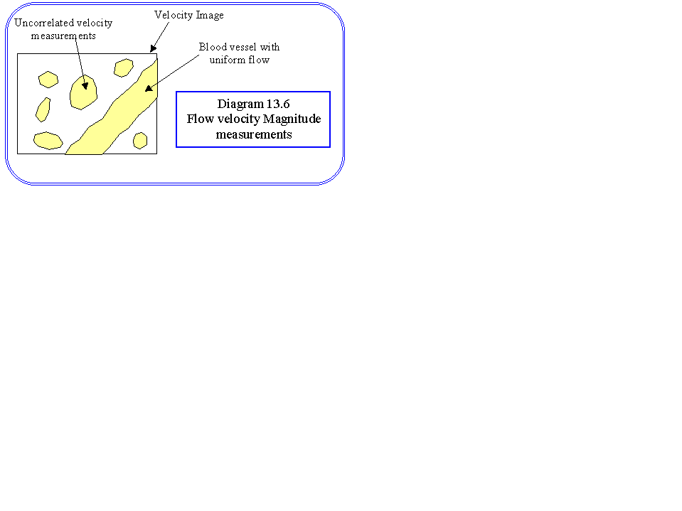
Magnetic resonance imaging has become very popular over the last few years, despite the huge cost of the equipment. Like CT the technique can measure densities so that bones and nuclear structures can be seen. The actual images do differ from the CT ones and often both techniques are required to complete a diagnosis. Alternatively, the technique can measure fluid velocities in slices through the body. This is particularly useful in diagnosing vascular diseases, such as restricted arteries. The image pixels that are passed to the computer for processing have an intensity proportional to velocity in a certain direction. Three images of the same slice create a complete velocity map, from which the artery under investigation must be identified, and its width and flow velocities measured. Unfortunately, in addition to the flowing blood, the image is confused by random noise caused by the other tissue (Diagram 13.6).

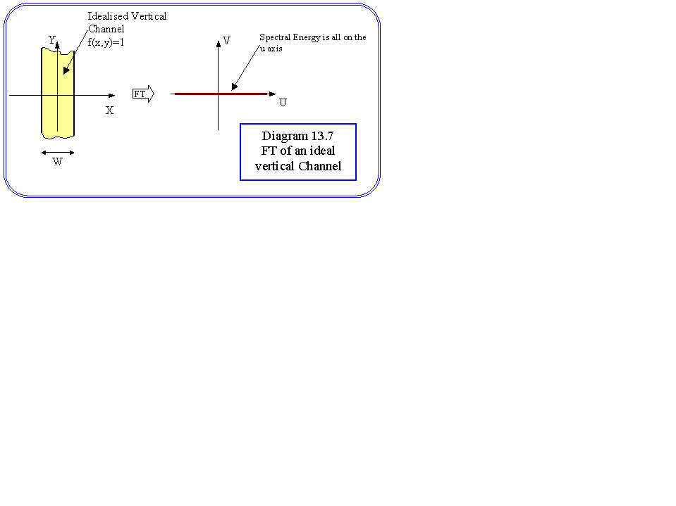
The invariant properties of the Fourier transform can help to solve the problem. To see how, first consider the transform of a vertical channel, specified by:

where w is the channel width. By evaluating this transform, we find that the spectrum has maxima along the u axis. Moreover, the invariance to shifting that we saw in the one dimensional transform also applies. Shifting the channel to the left or right merely applies a phase change to the spectrum, the magnitudes remaining unchanged (Diagram 13.7).

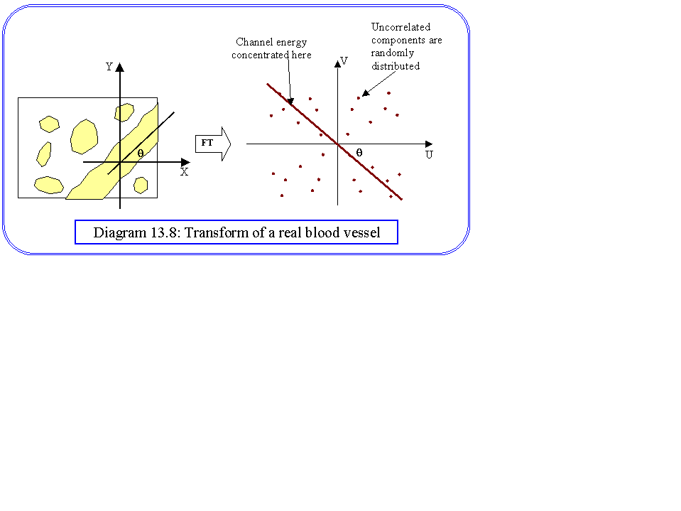
Thus, if the blood vessel we are examining has flow velocities predominantly in the vertical direction, it will show up as a channel in the vertical direction in the image whose equation will be approximately that given above. Hence it will produce maxima along the u-axis. The real image will have plenty of other features in the spectrum because of the noise, but will have a predominance of maxima on the x axis. Next, we remember the property that the spectrum preserves a rotation of the original image. Thus, if the vertical channel is rotated through an angle q, then the maxima in the spectrum will lie on a line through the origin, but at an angle q to the x axis. Hence if we fit a line through those maxima, we can estimate the angle of the channel. We can also estimate whether a channel is likely to exist from the strength of correlation in the frequency domain (Diagram 13.8).

Having estimated the angle of the channel, which gives us the direction of blood flow, we can return to the spatial domain, and eliminate all points which do not correspond to that flow direction, and this effectively eliminates the noise. Any noise remaining can be seen as isolated points and eliminated. The process is carried out in small windows to avoid problems of the arteries changing direction. Notice that we could do the whole process by correlation in the spatial domain, but to do so would require checking all possible flow directions. Since this is a three dimensional problem, two angle ranges would need to be checked. The use of the Fourier domain to estimate the flow direction greatly reduces the computation required. In practice it is possible to implement the algorithm entirely in the spatial domain.