Quantum Circuits
on a Parallel Machine
Individual Project
FINAL REPORT
Jonathan Marshall
MEng IV
Supervised by Steve Vickers
Modern microprocessors have to be designed with quantum mechanics in mind in order to ensure that they function correctly. In essence they use quantum effects to ensure that their classical computations are upheld. What no current processor does is to fully exploit quantum effects. Recently, it took 1,600 computers communicating over the Internet 8 months to solve the factorisation of a 129-digit number. Should it be possible to build a microprocessor which fully exploits quantum mechanics then it may be possible to carry out such factorisations in remarkably less time. The RSA algorithm, a widely used encryption system, is safe only if such factorisations cannot be performed quickly.
This report details a successful attempt to build a quantum circuit simulator. The project was undertaken as part of a final year assessment for a MEng degree in Computing at Imperial College, London. The simulator can accurately simulate circuits that are far more complex than anything that is expected to be built within the next few years.
The simulator runs on an IBM compatible PC running Windows NT or Windows 95. It takes an input in the form of a mathematical description of a circuit and then simulates it. It appears that this report is the first report on an attempt to build a quantum circuit simulator and the simulator itself may well be the first one to be publicly released. Due to this I have had to invent a number of algorithms for use in simulating the circuits. These algorithms are documented with the main body of this report.
Quantum computation appears to be inherently exponential in space and time to simulate on a classical machine and so the field of quantum circuit simulation is rich in possible heuristics that may reduce the resource requirements. I have made a start on researching such heuristics and the results are documented within.
This report also attempts to explain the behaviour of quantum computation and why it allows the possibility of exponential speed-ups over classical machine to the lay person. Later sections of the report document my design and implementation of the simulator in roughly chronological order and my thoughts on modern design processes. This may be of some interest to computing professionals.
I would like to thank Iain Stewart for introducing me to the field of quantum computation in the first place, suggesting an excellent project idea and then explaining the basics of the field in such clear terms. I would also like to thank my project supervisor, Steve Vickers, for his help and guidance throughout the course of the project.
The works of P W Shor, David Deutsch and many others have provided the central research material for this project. Without their constant research in to this exciting field projects such as this would not be possible.
Abstract *
Acknowledgements *
Contents *
Introduction *
Background to Quantum Computing *
Introduction to Quantum Effects
*Quantum Gates
*Reversible Computations
*Potential & Problems
*Fast Quantum Algorithms *
Factorisation Of Numbers
*The Simulator’s Final Design *
Matching of the Simulation to the Initial Specification
*Design and Implementation *
Design Methodology
*Initial Overall Design
*Platform Decision
*Initial Front End
*Initial Simulator Design
*Mathematical Classes
*Core Components
*The ‘Simple’ Simulation Algorithm
*Haskell
*Optimised Algorithms
*Testing
*Conclusions And Future Work *
Bibliography and References *
Appendix *
Class Overview diagram
*Class Reference
*User Guide For Quantum *
Installation
*The Quantum Application
*Performing a Basic Simulation
*Performing a Quantum Factorisation
*Menus
*Simulation Options
*Simple Test Circuits
*Automated Testing (Debug Version Only)
*Selected Source Code Extracts *
CIRCUIT.HS
*GATES.HS
*
In the early 1980s Richard Feynman [Feynman, 1982] noted the simulation of quantum mechanical systems always seemed to require a large amount of time and memory, with the amount being exponential in the number of quantum variables in the system. If it could be proved that this was always the case then this would open up the possibility of great speed increases for our computers. For instance, suppose a quantum system takes ten steps to perform some task and the simulation of this task requires a million steps. The simulation is nothing more than a large number of calculations. This then implies that there are some calculations that always take a million steps to perform on a ‘classical’ computer but which would require a mere ten steps in a quantum system.
This opens up the possibility of quantum computers – computers whose circuits act in such a way as to fully exploit the mysterious world of quantum physics. These computers, should we be able to ever build them, would allow a large speed increase over our current computers for certain types of tasks.
Quantum physics and the background to quantum computation is discussed in the section entitled ‘Background to Quantum Computing’. The ‘Potential & Problems’ section covers areas where quantum computers may offer a speed increase over quantum computers and also notes some of the problems in building quantum circuits.
This project aimed to provide a quantum circuit simulator. The simulator takes an input describing a quantum circuit, simulates the circuit and outputs the result that an idealised quantum circuit would output. The simulator allows researches in to the field of quantum computation a tool for verifying the correctness of quantum circuits. Currently only other way to simulate a quantum circuits is to model the circuit mathematically – the simulator allows researchers to change values and experiment with circuits in a much more flexible manner
The simulator makes no attempt to model the intricacies of quantum field equations. Instead it takes a ‘black box’ approach with quantum gates, the building blocks of quantum circuits.
My highest priority in this project was to produce a working and accurate simulator. Secondly I wanted to optimise the simulation so that it would maximise the potential of the computing resources available to it.
The original specification of the project and a comparison with the final product is available in the section ‘The Simulator’s Final Design’. The ‘The Design And Implementation’ section documents the decisions made throughout the project. Within this section is a sub-section entitled ‘Optimised Algorithms’ which details my research in to optimised simulation algorithms. Finally, the Appendix gives an overview of the objects used within the implementation of the simulator.
This report and the source code for the project is available online at
www-students.doc.ic.ac.uk/~jim1.
Background to Quantum Computing
Introduction to Quantum Effects
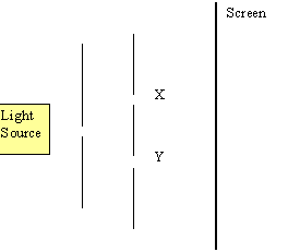
In Young’s double slit experiment below (Figure 1) light coming from the light source produces interference patterns on the screen S. If we were to consider that light is a wave then the patterns can be explained by the interference of light travelling through slits X and Y.
Since Young first performed his experiment in 1801 we have gained a far better control over our light sources. We also now know that light is made of particles called photons. We can arrange for a single photon to leave the emitter, pass through the slits and hit the screen. What we see is that the photons strike certain areas of the screen more often than other areas, and that that this is the reason for the light and dark fringes.
This raises some interesting questions. For instance, just why does a single photon hit the screen more in some areas than in others? If light is made up of particles then how can a single particle travelling through one of the slits X or Y produce an interference pattern? As only one particle has been emitted from the light source surely there is nothing for the particle to interfere with.
One theory is that the photon is more likely to strike certain areas of the screen because it has effectively travelled to the screen via every possible path, with some paths interfering with others. This interference may be constructive or destructive and accounts for why the photons never hit certain areas of the screen. The effects of quantum interference are even more apparent in the results of a second experiment, shown below.
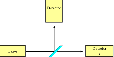
Consider a beam of light being emitted from a laser and hitting a partially reflective mirror, as shown in Figure 2. The mirror has been designed to reflect or transmit light with equal probability, so 50% of the light will hit detector 1 and 50% will hit detector 2.
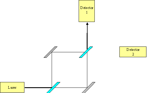
Now consider an attempt to recombine the beam, as shown in Figure 3. The paths are set up to be exactly equal in length. What we find is that 100% of the light hits detector 1.
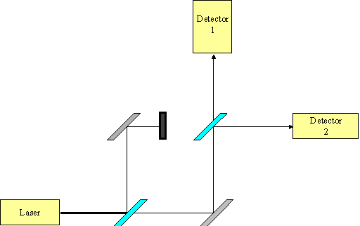
Now consider the same experiment with one of the paths blocked, as in Figure 4. What we now find is that 50% of the light hits detector 1 and 50% hits detector 2. Again we can adjust the light source so that only 1 photon is emitted at a time and again we find that this single photon behaves exactly as it would if it was a wave. In Figure 4 we know which path the electron has travelled as one of the paths is blocked. Yet how does this single photon know that this blockage on a remote path exists and that, with such a blockage, it must act differently when it reaches the second partially mirrored surface?
Again it seems that we must accept the result that at the quantum level particles do not travel single paths, instead they travel to their destination by every possible path. Although this seems counterintuitive this area of quantum physics predicts measurements that agree with our observations to an astounding degree. For a more comprehensive explanation of the basic theory of quantum mechanics read Richard Feynman’s excellent book, QED: The strange theory of light and matter.
If a photon travels to a destination via every possible path then can we use this quantum behaviour to our advantage in computing? It is clear that the universe is performing far more work in calculating the destination of a photon than one would expect from a classical point of view. As our machines are based on classical ideas of mathematics can this extra work by the quantum universe be converted in to extra computational power for our machines? The answer would appear to be a yes.
It was Benioff [1980, 1982a, 1982b] who showed that a machine whose computations were performed according to the laws of quantum mechanics physics would be at least as powerful as a classical Turing machine. It was Richard Feynman [1982, 1986] who first postulated that a quantum mechanical system takes an exponential amount of time to simulate on a classical machine. This then implies the reverse - that some computations which take an exponential amount of time to run on a classical machine can be computed in polynomial time by a quantum mechanical system. It was David Deutsch [1985, 1989] who was the first person to seriously investigate this possibility and define a Quantum Turing Machine.
Many Worlds Formulation
In one formulation of quantum theory, the Many Worlds interpretation, there are actually many copies of the universe which have certain probabilities of existing. In each universe the photon travels to its destination along one path. The interference that we see on the screen is due to the universes constructively and destructively interfering with one another. The universes where the photon strikes a dark patch of the screen have little possibility of existing while the universes with light patches have a reasonable chance of existing.
The Many Worlds theory originated with Dr Hugh Everett, III, is supported by some of the leading investigators in the field of quantum computation. The following in an extract from the "Many Worlds" faq by Michael Clive Price, which is available online.
"Political scientist" L David Raub reports a poll of 72 of the "leading cosmologists and other quantum field theorists" about the "Many-Worlds Interpretation" and gives the following response breakdown.
1) "Yes, I think MWI is true" 58%
2) "No, I don’t accept MWI" 18%
3) "Maybe it’s true but I’m not yet convinced" 13%
4) "I have no opinion one way or the other" 11%
Amongst the "Yes, I think MWI is true" crowd listed are Stephen Hawking and Nobel Laureates Murray Gell-Mann and Richard Feynman. Gell-Mann and Hawking recorded reservations with the name "many-worlds", but not with the theory’s content. Nobel Laureate Steven Weinberg is also mentioned as a many-worlder, although the suggestion is not when the poll was conducted, presumably before 1988 (when Feynman died). The only "No, I don’t accept MWI" named is Penrose.
The Many Worlds theory allows us a view of the behaviour of quantum computation which some find easier to visualise. The theory does differ from other quantum theories in its predicted results in certain areas. This opens up the possibility of being able to disprove the theory one day. Deutsch [1985] describes one possible experiment using an artificial intelligence computer built using quantum circuits. This experiment is currently far beyond our technical expertise.
The theory implies that there are many copies of you in many different universes. We are not aware of other copies because there can be no communication between the universes. This is disconcerting to a number of people who do not like their individuality to be impeached upon.
For the remainder of this text the Many Worlds theory shall be the only one used in explaining the behaviour of quantum circuits.
Imagine a hydrogen atom in its ground state. If we supply an amount of energy at the correct frequency for a certain period of time the atom will become excited. If we supply the energy for only half of this period then the atom will be in a superpositioned state - that is in some universes the atom will still be in a ground state and in other universes it will be in an excited state. Note that the particle is not in some intermediate state - it is definitely in one state or the other and measuring it will tell you which state the particle occupies in your universe. An otherwise identical copy of you in a different universe will have performed exactly the same measurement and will have seen the opposite result.
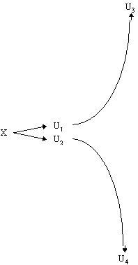
Again consider a particle in its ground state in universe X. Again we supply the correct amount of energy so that the particle enters a superpositioned state. The universe X will then split in to two universes: in universe U1 the particle is excited and in universe U2 the particle is still in its ground state. In all other aspects these two universes are absolutely identical. We can see this in Figure 5 where time increases along the x-axis.

Each of these universes will have an amplitude attached to it. The amplitude is a complex number that corresponds to the likelihood of that universe existing. What we would term as being the probability of the universe existing is the magnitude squared of this complex number, which obviously must lie on or between 0 and 1.
Now if we consider the above example again, what would happen if there was another route for the universe U1 to be created, as in Figure 6. Here universe Y can also split in to two universes, one of which is identical to U1. It is obvious that the probability of U1 occurring must now be affected as there are two paths leading to this universe. This is not to say that the probability of U1 increases. The amplitude of U1 is determined by the a mathematical combination of the amplitudes of X and Y and of the amplitudes of X leading to U1 and Y leading U1. As amplitudes attached to these universes and actions are complex and may well involve negative numbers the probability of U1 existing may well be less in this example than it was in the previous example. Hence the universe may well destructively interfere as well as constructively so, and this is why we see dark fringes in Young’s double slit experiment.

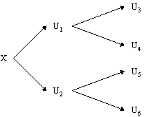
It is important to note that the universes must be absolutely identical for interference to occur. Again consider a particle in a universe X which is then transferred in to a superpositioned state in universes U1 and U2. Now we measure the particle. In universe U1 you would see that the particle is excited and you and the particle would enter universe U3, and in U2 you would see that it is in the ground state and enter universe U4. By this process of measuring the state of billions of particles in your brain have been affected. The difference between U3 and U4 would not be one particle, as with the differences of U1 and U2, but billions of particles. U3 and U4 would be so far apart that there would never be any hope of the two universes becoming identical at some point in the future. Thus they will never interfere again. We call this process decoherence, and it can be seen in Figure 7 with the y-axis representing a qualitative measure of the distance between universes (that is to say how different they are).
Qubits
We define a quantum bit (Qubit) as being a particle in the superposition of two values, which we will denote |0> and |1>. Here we use the ket notation |> to remind us that we are dealing with quantum systems and not classical ones. For instance, we could denote the excited state of a superpositioned particle as being |1> and the ground state as being |0>.
Let’s place a particle in to the superposition of two values, |0> and |1>. Again we get two universes, each with an assigned amplitude. If we were to then to place another particle in a superposition of two values we’d then get four universes, as shown in Figure 8. If we were to repeat this process then we would get eight universes, and so on.
In fact for n superpositioned particles in two possible states we get 2n different universes with every possible combination of the n particles values being observed. As with classical machines we can call a collection of bits a register. However, the difference is that a classical register can only hold one value. A quantum register of length n bits can hold up to 2n values simultaneously with each value observed in an otherwise identical universe. This quantum register could be used as the input to some circuit. The circuit will then act simultaneously on these 2n different inputs, perform 2n different calculations and output 2n superpositioned results. This is the source of the exponential speed-up of quantum computers, and has also been dubbed parallel processing on a serial machine. In essence, for the cost of building only one circuit we can have the circuit perform an exponential number of calculations simultaneously.
The trick is to get all of these universes to interfere with each other in such a way as to produce an output that is of some use to us. Consider the situation where we have the functions in the 2n universes outputting a different value with equal probability. If we were to perform a measurement on the output value the systems would decohere and the value read would be a random value from the 2n outputs, which wouldn’t really tell us very much. What’s required is to arrange for the universes to interfere with each other with each other in such a way so that the output value(s) of interest have a much higher probability of being observed and, conversely, those values which are not of interest having a much smaller probability of being observed.
This leads to an interesting question. If we require that the output from a quantum circuit interferes in such a way as to make certain outputs being made more probable than others, then does this lead to a restriction on the type of class of problems which quantum circuits could perform more efficiently than their classical counterparts? Would it lead to a more efficient algorithm but with a less than exponential speed up? This question is analogous to the question of whether parallel processing machines can effectively speed up all problems or whether there are some inherently sequential problems that refuse to yield to parallel techniques. The answer to this question on quantum computation would appear to be yes, there is a limit to what quantum computation can speed up. The section Potential & Problems later gives an overview of some of the early results in the field of quantum complexity analysis.
It appears that the laws of physics are completely reversible. That is, from any physical process we can always deduce the inputs from the outputs. Classical computers would at first appear to violate this law as we can easily create functions on classical computers that are not reversible. For instance consider the Boolean AND gate, the truth table for which is shown in Figure 9. There is no way of completely deducing the inputs of an AND gate from the outputs, and thus the AND gate appears not to be reversible.
|
Input 1 |
Input 2 |
Output |
|
0 |
0 |
0 |
|
0 |
1 |
0 |
|
1 |
0 |
0 |
|
1 |
1 |
1 |
The answer to this riddle lies in waste heat. An AND gate in a classical computer produces waste heat as well as its intended output. The ‘lost’ information about the inputs contained in this waste heat.
In quantum computers, we cannot allow this situation to occur. The radiation of the heat would depend on the state of the inputs to the quantum gate. Thus, in effect, the radiation of the heat would be a measurement on the inputs and decoherence would ensue. The universes would be so far apart as to be unable to interfere with each and the result, which depends upon the interference of these universes, would be invalid. Thus quantum gates must be reversible. Reversible gates must, by their very definition, have an equal number of inputs and outputs.
Gates are called universal gates if they can be used to create any logic circuit, such as the NAND gate in classical circuits. Three other examples of universal gates are the Universal Toffoli gate, the Fredkin gate and the controlled NOT gate. These gates have the advantage that they are reversible as well as universal.
The Universal Toffoli Gate has three inputs. The first two inputs are copied to the first two output pins and the third output is the Exclusive OR of the third input and the AND of the first two inputs, as shown in Figure 10.
|
Input 1 |
Input 2 |
Input 3 |
Output 1 |
Output 2 |
Output 3 |
|
0 |
0 |
0 |
0 |
0 |
0 |
|
0 |
0 |
1 |
0 |
0 |
1 |
|
0 |
1 |
0 |
0 |
1 |
0 |
|
0 |
1 |
1 |
0 |
1 |
1 |
|
1 |
0 |
0 |
1 |
0 |
0 |
|
1 |
0 |
1 |
1 |
0 |
1 |
|
1 |
1 |
0 |
1 |
1 |
1 |
|
1 |
1 |
1 |
1 |
1 |
0 |
The Fredkin gate has three inputs. The last two inputs are swapped if the first input is 0 and is left untouched otherwise, as shown in Figure 11.
|
Input 1 |
Input 2 |
Input 3 |
Output 1 |
Output 2 |
Output 3 |
|
0 |
0 |
0 |
0 |
0 |
0 |
|
0 |
0 |
1 |
0 |
1 |
0 |
|
0 |
1 |
0 |
0 |
0 |
1 |
|
0 |
1 |
1 |
0 |
1 |
1 |
|
1 |
0 |
0 |
1 |
0 |
0 |
|
1 |
0 |
1 |
1 |
0 |
1 |
|
1 |
1 |
0 |
1 |
1 |
0 |
|
1 |
1 |
1 |
1 |
1 |
1 |
The Controlled NOT gate has two inputs. The second input is negated only if the first input is true, as shown in Figure 12.
|
Input 1 |
Input 2 |
Output 1 |
Output 2 |
|
0 |
0 |
0 |
0 |
|
0 |
1 |
0 |
1 |
|
1 |
0 |
1 |
1 |
|
1 |
1 |
1 |
0 |
The controlled NOT gate has attracted much interest in the field of quantum computation as it is reversible while requiring only two inputs. The difficulty of building a quantum gate greatly rises with the number of inputs to gate. The proof that two input gates are universal for quantum circuits has brought the possibility of building a quantum computer one step closer [DiVincenzo 1995].
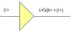
The square root of NOT gate is the first purely quantum gate that we shall examine and, from a classical point of view, is unusual in its behaviour. A single square root of NOT gate produces a completely random output with equal probabilities of the output being 0 or 1. However two such gates linked sequentially produce an output that is the inverse of the input, and thus behave in the same way as the a classical NOT gate.
This result is unparalleled in the classical world - one gate produces a random result while two gates linked sequential produce a deterministic result.
The truth table for the square root of NOT gate is shown below.
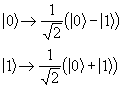
An input of |0> leads to an equal and opposite amplitude of the output being |0> or |1>. An input of |1> leads to a equal amplitude of the output of the gate being |0> and |1>.
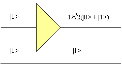
Now lets see what happens when we join two of these gates, X and Y, together. As shown in Figure 13.
Let’s say that the input to the first gate is |1>. The universe will split in to two universes, identical in every respect expect that the output to the first gate (X) is |0> in one universe and |1> in the other universe. Lets consider the |0> part of the superposition. This will get transformed in to
![]()
and the |1> portion of the superposition will get transformed in to
![]()
The total state of the system is then:
![]()
Note that the possibility of the output of the system being |1> is cancelled. Here you can see the interference of the quantum universes working. The universes can only interfere because they are identical in every regard except for this superpositioned particle. Suppose that we were to place a detector at M to tell us the value of the output to gate X. One copy of ourselves would note that the value is 0 while another copy in a different universe would note that the value is 1. Thus the universes would be different by billions of particles and could never again interfere. So just to know the value of the output of X invalidates the output of gate Y, even if our detector could measure the output of X accurately without disturbing the system.
The requirements for reversible gates have been shown above. Without such gates the quantum system would radiate heat and the quantum interference which is essential for the correct operation of the system would stop working. However it is not enough to simply have reversible gates - the entire computation must be reversible. What’s more, we cannot copy or destroy values within the system without it decohering. The classical instructions X:=Y and X:=0 lose information as the original value of X is obliterated by the instruction. Thus they are not reversible, and so could never be used in a quantum computation algorithm. Instead we need to replace those instructions with variations such as X:=X + Y (where we know that the original value of X was 0) and X = X - Z (where we have computed that the value of X is Z).
Thankfully it has been shown [Lecerf 1963, Bennet 1973] that any deterministic computation can be made reversible.
Gate arrays are acyclic circuits. If we are allowed a small probability of error, quantum gate arrays and quantum Turing machines can compute the same functions in polynomial time [Yao 1993].
It’s far easier design a reversible circuit if it is gate array and so this tend to be the form of quantum circuit used most frequently in the literature.
The potential of quantum circuits is easy for all to see. It offers the promise of an exponential speed up over classical machines for a certain group of problems. The problems known to date to have fast quantum algorithms are listed below.
Limits
Researchers are currently looking in to the classes of algorithms of quantum computers. The computational class BPP is widely regarded as the class of efficiently solvable problems on a classical computer. The class BQP is the analogue for quantum computers. It is not known whether BPP º BQP, and indeed it is not possible to solve this conclusively without answering the major open problem P º PSPACE? There is some evidence though that BPP ¹ BQP [Bernstein and Varirani, 1993], and thus that quantum computers do offer a real speed up over their classical counterparts.
There have been proofs published [Bennet et al, 1996] which show that quantum computers cannot solve the class NP with more than a quadratic speed up over their classical counterparts. This is less than the exponential increase that we would desire, though it still offers dramatic increases in speed.
Physical Problems
The possible advantages of quantum computers balanced the disadvantages in building the device. Remember that a measurement on a superpositioned value will lead to decoherence, and that the resultant universes after decoherence will never again interfere with each other. The output to a quantum circuit depends on quantum interference, thus performing a measurement on a quantum circuit will result in the output to the circuit being incorrect. What then is a measurement? We can simply think of a measurement as being an interaction of the superpositioned particle with some other particle. Thus a stray molecule colliding with the superposition particle or light shining on the particle could be enough to destroy the computation. This means that the creation of a quantum circuit consisting of many thousands of gates would be fiendishly difficult. The creation of just two quantum bits by Chris Monroe and his team from the National Institute of Standards and Technology involved the trapping of an ion in a magnetic field and then cooling it to near absolute zero.
Further problems stem from the fact that trying to copy a quantum bit would inherently involve a measurement of the bit. The copying of data is inherent in classical error correction systems, and it would seem that quantum computers would require error correction far more than classical computers ever would.
Yet there is hope. P. W. Shor recently invented an error correction mechanism that involves using an extra eight bits of redundant data for every bit in the circuit. Researchers at IBM, Los Alamos and Oxford then managed to reduce this down to an extra four bits. The error correcting mechanism works by encoding five qubits from a single input bit. If a measurement is later carried out on a single bit then this does not give away enough information to reveal the contents of the other four bits. The error can then be later corrected. The down side to this is of course that it requires the quantum circuit to consist of far more gates than before.
Hope also comes from Shor’s work on the reliability of large quantum systems. Von Neuman in "Synthesis of Reliable Systems from Unreliable Parts" showed that one does not need components which are more reliable in order to run a longer classical computation - one just needs to slow the computation down to allow for error correction. Original detractors of computers had believed that to increase a computation length by x times one would require components which were x times more reliable. Shor has not managed to duplicate this result for quantum circuits, however he has managed to show that increasing the length of a quantum computation by x times requires a constant increase in the reliability of the components, not a factor of x.
Moore’s Law states that microprocessors will double in the number of gates every eighteen months. Today, nearly thirty years later, this law is still holding strong. Yet even Moore himself believes that we will not be able to carry on at such a rate for another thirty years. In the future we will need to design a radically different technology if we are to continue growing our computer’s performance at such an exponential rate. Perhaps quantum computation is the technology to achieve that goal.
Nobody really believes that we will have mass-produced quantum processors on our desktop any time soon. The physical difficulties of manufacturing a reliable large quantum device are far beyond are current technical expertise. But perhaps we should remind ourselves that the possibility of creating computer gates of 1 micron in size would have been described by many as physically impossible just fifty years ago, yet today one can stop off at a local computer store and casually buy a six million gate microprocessor with gates of just 0.35 microns in size for less than a hundred dollars. What once seemed impossible is now reality. Perhaps the techniques will be found to mass-produce quantum microprocessors within the next fifty years.
Even the detractors of quantum computation are willing to acknowledge one thing. The discussion and research in to this field has served to remind us that mathematics is not an abstract art. Instead it is firmly based in the reality of the Universe. The theories of quantum computers have served to remind us that computation is a physical process, bound by the laws of physics. Hence to achieve the maximum computational speed one must fully exploit the laws of nature.
Given a number which is the multiplication of two prime numbers (a co-prime) then can you work out the two primes that were used in the multiplication? The problem can easily be reduced to working out one of the prime numbers as a simple division would then lead to the other number. The factoring of numbers is of intense interest in the field of cryptography. The RSA algorithm, the most widely used public key cryptosystem, is used by many World Wide Web browsers for the secure transmission of sensitive information such as credit card numbers. The algorithm is secure only if the factorisation of large numbers requires a super-polynomial amount of time with respect to the size of the number. To date it has not been proved that the process of factorisation of numbers requires an exponential amount of time. However no classical polynomial time algorithm has been found and researchers generally believe that none will ever be found.
Best Classical Factorisation
The best known classical method for factoring numbers is currently the number field sieve [Lenstra and Lenstra, 1993]. It has an asymptotic run time of approximately ![]() , where n is the number to be factorised. As the length of the number n is O(ln n) this means that the factoring algorithm is exponential in the length of n. The factorisation of a 512 bit number using this method requires approximately 1019 steps.
, where n is the number to be factorised. As the length of the number n is O(ln n) this means that the factoring algorithm is exponential in the length of n. The factorisation of a 512 bit number using this method requires approximately 1019 steps.
Quantum Factorisation
This uses an algorithm described in [Shor 1996] and has an asymptotic run time of approximately ![]() steps on a quantum computer. Let n be the number that we are trying to factorise. Let x be a random number and let a be a number which ranges between 0 and q-1, where q is a power of two such that n2 £
q £
2n2. Then the sequence xa (mod n) will have a certain period. Let r be the period, then one of the factors of n is the greatest common divisor of xr/2-1 and n.
steps on a quantum computer. Let n be the number that we are trying to factorise. Let x be a random number and let a be a number which ranges between 0 and q-1, where q is a power of two such that n2 £
q £
2n2. Then the sequence xa (mod n) will have a certain period. Let r be the period, then one of the factors of n is the greatest common divisor of xr/2-1 and n.
As an example, suppose we are trying to factorise the number 33 and that we have chosen the random number 5. The start of the sequence xa (mod n) is shown below,
|
a |
xa |
xa (mod n) |
|
0 |
1 |
1 |
|
1 |
5 |
5 |
|
2 |
25 |
25 |
|
3 |
125 |
26 |
|
4 |
625 |
31 |
|
5 |
3125 |
23 |
|
6 |
7825 |
16 |
|
7 |
390625 |
4 |
|
9 |
1953125 |
20 |
|
10 |
9765625 |
1 |
|
11 |
48828125 |
5 |
|
13 |
244120625 |
25 |
|
14 |
1220703125 |
26 |
As you can see the sequence 5a (mod 33) repeats itself after 10 entries. The greatest common divisor between 55-1 and 33 is 11, which is a factor of 33. For the above algorithm to work n has to be odd and not a prime power, r has to be even and xr/2 (mod n) has to be not equal to -1. Although this may seem like a rather large number of constraints that are required for the algorithm to work the constraints, in practice, do not cause much of a problem. If n is even then finding a factor is trivial. If it is a prime power then classical methods will yield a factor quite efficiently. Otherwise it can be shown [Shor 1996] that a random choice of x will yield a correct result with the probability of 1 - 21-k, where k is the number of distinct odd prime factors of n. Hence a co-prime is likely to yield a correct factor 50% of the time with a randomly chosen x.
On classical machine the problem of finding the period of a sequence of number like xa (mod n) requires an exponential amount of time. However on a quantum computer we can perform the xa (mod n) in parallel and then perform a quantum Fourier transform to reveal the sequence.
The Quantum Fourier Transform
The details of the Quantum Fourier Transform (QFT) are mentioned in detail in Shor [1996]. To summarise, a series of gates is applied to an input. Each input value if mapped to the value 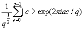 , where q is 2n, n is the number of bits in the QFT, a is the state being mapped and c is the state that it is mapped to.
The Quantum Factoring Algorithm
The algorithm itself is relatively straightforward. Take a quantum computer and divide its bits up in to two registers. Place the bits of the first register in equal superpositions of the values 0 and 1. Then set the second register as the value xa (mod n), where a is the value in the first register, x is a random number and n is the number to factorise. Perform a quantum Fourier transform on the bits in the first register and then observe the result. The probability of observing a value in the first register will, if all goes well, be something like the graph shown in Figure 14.
The value of r, i.e. the period of xa (mod n), is the number of peaks in the output. In a quantum circuit we would not observe the entire output, only one random value. However there are far higher chances of seeing certain values (thanks to the interference) and so we can be sure that after a few iterations of the circuit we will obtain enough information in order to deduce r. A factor of n is then the gcd(xr/2-1, n). In the above graph n is 33, x is 211 and r is 10, leading to a factor of 3.
Comparison Of Classical And Quantum Factorisation
A comparison is best illustrated by a graph of the run times of the two algorithms.
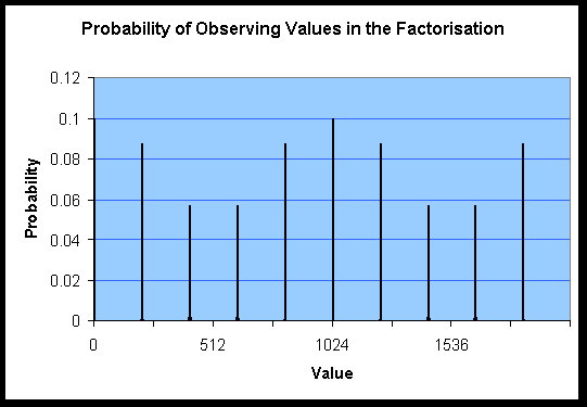
As you can see from the above graph factoring a 512 bit number requires something on the order of 1015 times more steps using a factoring algorithm on a classical machine than using a factoring algorithm on a quantum circuit. This is why there is so much interest in the field of quantum computation. Even if decoherence problems mean that a quantum circuit may only work correctly one in every thousand times and even if the operation of each gate in the quantum circuit was a thousand times slower than classical gates the factorisation of a large number would still be many orders of magnitude faster on a quantum computer than it would be on its classical counterpart.
Matching of the Simulation to the Initial Specification
This section of the report compares the current features of the simulator to those that I set out in the simulator’s initial specification. To summarise, all major requirements of the specification have been met and a number of requirements have been exceeded. The simulator accepts input files, runs and produces valid output. The differences between the specification and the implementation are mainly concerned with the smaller issues which I did not have time to research fully before the specification had to be completed. Thus the spirit of the specification is upheld, while the letter may not be.
For a fuller discussion of the decisions not to adhere to the letter of the specification see the Design and Implementation section. Where the implementation differs a brief reason for the difference is outlined here.
For your convenience excerpts from the initial specification are quoted.
General
The simulator will take an input describing the circuit to be modelled, ask for any parameters required for the simulation, run the simulation and output an accurate set of results. It is absolutely essential that the output is correct under all circumstances.
The circuit to be modelled will be a quantum gate array, i.e. it must be acyclic. Each gate in the array must be reversible and have a fixed and equal number of inputs and outputs. All values in the circuit will be in binary. Amplitudes of events will be modelled by complex numbers. The inputs to the gate array may be fixed values, randomised values or superpositioned values.
All requirements were met. Superpositioned inputs were later removed from the project, see the Design and Implementation section of this document for the reasons as to why. This does not affect the operation of the circuit as a superpositioned inputs can be emulated by following a fixed input with a Square Root of Not gate. All simulations appear to give the correct results.
The program should take an input file describing the circuit to be modelled. The file should be in text format. In the input file it should be possible to define the number and type of input and output connections, define new gates, declare the gates to be used in the simulation and specify the connections between gates. The syntax of the input file should be easy to learn.
The input connections to the circuit should include superpositioned inputs with equal probability of bits being 0 or 1, random inputs and inputs whose value can be set to certain values. Such inputs have proved to be useful in quantum circuits.
The program should detect and reject invalid inputs. In particular it should reject the declaration non-reversible gates (the matrix for a quantum gate must be unitary, i.e. inverse is its conjugate transpose). It should also reject invalid circuits where the user has attempted to connect something more than once or something has been left unconnected. The circuit should be checked to ensure that it is acyclic. The simulator need not ensure that the circuit is reversible.
An example of an input file which is considered adequate follows:
include othergates.h
[CircuitSize]
superpositioned inputs = 2
random inputs = 3
standard inputs = 2
outputs = 3
[NewGate]
Name = StrangeGate
inputs = 2
MatrixRow1 = 1, 0, 0, 0
MatrixRow2 = 0, 0.3 + .2i, 0, 0
MatrixRow3 = 0, .5, .5, 1
MatrixRow4 = .2, .2, 0, 0
[Gates]
SquareRootOfNOTGate = a, b
StrangeGate = c
[Connect]
StandardInput.1 -> 0
SuperInput.1 -> a.Input.0
random.2 -> b.Input.0
a.Output.0 -> Output.2
All areas of the above specification were met (with the exception of superpositioned values noted above). However it was decided to change the input format considerably from the example given above to one which would give far more flexibility and power. The bare format to the simulator has been changed to a series of complex numbers. Admittedly such an input format could not be described as easy to learn. However, a functional programming language can easily generate such a series of numbers. This has the advantage of allowing the user to specify a circuit programmatically. As the vast majority of useful circuits can be specified recursively this enables a compactness of code which would not be achieved otherwise. My implementation of a circuit to perform a quantum Fourier transform, an important subroutine involved in factoring numbers, takes a mere 50 lines in Haskell - no matter how many bits are desired in the input to the circuit. Using the example above format would have required a different input file for each size of circuit, and the size of an input file describing a circuit which operates on sixteen input bits would require over 300 lines of code.
The simulator now expects the user to specify input files in Haskell and provides facilities to running a Haskell interpreter. Again, see the Design and Implementation section for more details.
After loading the input file the simulator should ask the user for any extra required parameters before starting the simulation. A progress bar should be displayed during the simulation and it should be possible to terminate the simulation gracefully.
The priority of the thread(s) on which the simulator is running should be adjustable by the user interface. It is expected that a complex simulation may take several hours to run, and it would be useful to make sure that the machine is not unavailable for other uses during this time.
All of the above requirements were met.
A quantum circuit will not produce one output value. Instead, all possible values are output with each value having a certain probability of existing.
The system shall have two modes of output. In the first mode all possible output values will be output together with their probabilities. Obviously, for n outputs, this entails a table of length 2n. An example is given below:
|
Output 0 |
Output 1 |
Real Probability |
Complex amplitude |
|
0 |
0 |
.5 |
.707 |
|
0 |
1 |
.25 |
.1 + .3i |
|
1 |
0 |
.25 |
.3 + .1i |
|
1 |
1 |
.0 |
0 |
The format of the output will be as above. Each output wire will have its own column in the table. The final column will be the complex probability of the values existing. The preceding column will be the real probability of the combination of output values existing, which is equal to the magnitude of the complex value squared.
In the second output mode, a number of values will be randomly selected in accordance with their probabilities. So if one output was to be randomly selected from the above example there would be a 50% chance of 00 being output and a 25% chance of 01 or 10. In this mode the user will simply get a list with the chosen outputs.
The simulator will ask the output mode and the number of values to select before the simulation starts. The output should be dumped to a user selected file, or viewed on screen.
Cosmetic changes were made to the output format specifications. The output is now a two column table. The first column is the value being observed in either binary or decimal, the second column is its complex amplitude or real probability. A circuit could well output millions of values and this format offers compactness over the above specification without losing any information.
The system does not output values randomly selected in accordance with their probabilities, although this feature would be trivial to implement. One of the few advantages of running a quantum simulator over running a quantum circuit is that you can observe every amplitude output by the circuit. Whereas with a quantum circuit you can only observe one value every time you run the circuit.
A feature not originally specified is the histogram output, where the contents of a selection of bits can be observed. This is useful where the simulation models a circuit with a number of quantum registers.
The software should be developed on Windows NT machines using Visual C++ 4 and 32-bit code. The program will be required to work under Windows 95. As such the program will need to consist of a shell Windows interface which surrounds the core simulator.
Care should be taken that the core simulation code is reasonable easy to port to UNIX platforms. That is to say that there should be a clear dividing line which separates the Windows front end from the core simulation code, and that the simulation code should not depend on features specific to the Visual C compiler.
Resources
A simulation of a quantum circuit will be exponential in both time and space. While there is no hope of producing a system that can simulate a quantum circuit in polynomial time (such a simulator would in fact require a quantum circuit) care should be taken to minimise resource requirements where possible.
There are at least two areas where savings could be made. Firstly, there may be a large number of universes that have zero probability of existing.
Secondly, although the system will require an exponential amount of space it may be possible to reduce the amount of time required to access this space by ordering the space in such a way as to increase the number of cache hits and / or decrease the number of page faults.
It is not clear at the time of writing as to whether these two methods will lead to any real improvements in the execution time or reductions in space requirements. The two methods should be evaluated and an analysis included in the Final Report.
There simulator should not define inputs to the circuits as quantum bits as their values and probabilities are always known.
If a large number of universes have zero probability of existing then there is a possibility that sparse vectors could be used to reduce the memory requirements of the simulation. A goal of this sort type of algorithm would be to minimise the memory requirements at the expense of computation times. Sparse vectors have been implemented and have proved a success in certain types of simulation, reducing the memory requirements of large quantum factorisations by a factor of ten. The results are discussed in the Optimisation section.
I have implemented a cache-hit increasing algorithm. I dubbed it the ‘complex’ algorithm as it requires far more control logic that the original ‘simple’ algorithm. The results are poor on small circuit simulations but outstanding on larger circuits. The extra overhead of the control logic required to order the computations means that savings in waiting for cache misses are negated in systems with enough available physical memory for the simulation’s workspace. However, where the system requires some virtual memory the cache-hit increasing algorithm reduces execution time by anything up to a factor of five and by a factor of ten when multiple threads are used. Again, see the Optimisation section for a discussion of the results.
Quantum Bit Saving
Savings in the number of quantum bits that need to be modelled could leave to massive savings in resources. This should be possible by joining gates together in to more complex gates that perform the same task but without outputting the intermediate result. For instance, two square root of NOT gates perform the same operation as a single NOT gate, Connecting the two square root of NOT gates requires a joining wire, which will have to be a quantum bit. Is we were to replace the two square root of NOT gates with a single NOT gate we would not need to simulate the joining quantum bit, halving the space and time requirements of the simulation.
The simulator will be expected to make such resource saving transformations to the quantum circuit wherever possible, though it will not be expected to attempt to find the most efficient saving in the case where there are alternative transformations which could be made.
Multi-Threading
The simulator should make use of multiple threads in simulating, However at the time of writing the initial project proposal it was envisioned that the application should make use of parallel processors on a shared memory machine in order to reduce computation time.
Unfortunately analysis of the problem has since shown that parallel processing on a shared memory machine may increase the computation time. The biggest factor in affecting the speed of the program will be the time taken to access the data required for the calculations. As this data will be spread around an area of memory of exponential size the processor will be unlikely to make many cache hits, thus overloading the bus which connects the processor to the main memory. Adding another processor to an already overloaded bus would decrease the processing power, not increase it.
If an algorithm can be found to increase cache hits (see above) then multi-threading may lead to reduced execution times on a parallel machine.
Windows 95 cannot handle multiple processors and so this part of the project is not intended work on Windows 95.
Expected Circuit Size
To model the behaviour of a quantum circuit capable of factoring the RSA-129 number would require a machine with more bytes of memory than there are atoms in the universe, which is obviously beyond the scope of this project!
It is expected that a circuit with 20 quantum bits of information would require about something on the order of 16 Mb of memory so simulate, with the amount of memory required doubling with every extra bit of quantum information. An effective maximum circuit size would be about 26 quantum bits.
Testing
The program must cater for a series of automated sequential tests on a user-specified set of input files. This will help to ensure that the program has met its specification.
I decided not to write the simulator to accept a list of input files to test as it would be inherently difficult for the simulator to determine whether its output was correct or not. For example, suppose the simulator accepts an input file as a test. This simulation of the circuit is performed and an output is produced. For the simulator to know whether its output is correct or not requires the simulator to know what it should have outputted in the test. Thus it effectively needs two inputs, one is the circuit to test and the other is a mathematical description of the expected result. To be able to correctly interpret a mathematical description of the expected outputs of a circuit would have involved a substantial amount of programming in itself.
Therefore I decided to abandon the original approach in favour of directly programming a fixed number of tests and expected results in to the simulator. These fixed tests have a number of random variables involved in their construction which mean that are actually more than a hundred million different tests which can be created and executed. The fixed tests are designed to catch the most likely things that can go wrong in a circuit’s simulation. My justification for these fixed tests comes from the result - so far I have not discovered a case where the continuous execution of a reasonable number of tests has succeeded and other circuits have failed. Typically I allow the simulator to randomly build and test about two thousand circuits over a number of hours before accepting that a change to the simulator has not adversely affected its correctness. This corresponds to an error rate of less than 0.05%. The most elusive simulator error to date was highlighted after approximately two hundred tests.
The first step in designing a product is to decide which design methodology you are going to use. For the vast majority of computer applications it is hard to say that one correct implementation is better than another. There is always a certain amount of artistry involved and evaluating between two correct implementations usually requires subjective arguments based on the preferences of the evaluator. In my belief such artistry extends beyond the choice of implementation and in to the choice of design methodology. I may, for instance, prefer one method for developing a certain type of application while another person prefers another. In a project such as this where there is only one programmer involved I would say that the design methodology to use is the one that the programmer is most confident of achieving results with. The methodology in question does not have to agree exactly with any well-known methodology.
Personally, I feel most confident with my own "mixed" design methodology. It is based on years of experience as a programmer and consists of elements of a number of publicised methodologies. I will selectively use the objects of OMT, top-down and bottom-up design based on the current task to solve. Overall the development structure could be called evolutionary with some rapid prototyping. Most of the professional programmers that I know use some variation of the technique when designing small to medium sized applications. It allows the flexibility of matching a particular style to the task in hand.
Perhaps the best way to illustrate the method is to go through the design process of the project in roughly chronological order.
It has to be said that the design did not occur wholly before the implementation, rather it was an ongoing processing throughout the implementation. The separation of the design from implementation is something that is inherent to the Waterfall method of design - a method which is widely regard as a nice idea, and perhaps even the ideal, but not something that accurately reflects programming reality. A design is not properly assessed until it is implemented, by which time, according to the Waterfall method, it is too late to change the design. This is even more apparent in experimental projects, such as this one, where there is little readily available knowledge as to which project design is correct because nobody has implemented such a project before. My technique for designing this project, which I believe to be the best one for experimental, time constrained projects, was to design a part of the project, implement it, assess the design, redesign if necessary and then move on to the next part of the project.
It was immediately apparent that there would be two parts to the simulator. There would be the actual simulation code itself, which I called the core simulator, and there would be a front end to the simulator. It is the very nature of front ends that they usually end up machine dependent. The core simulator, however, had no need to be machine dependent. The decision was taken to try to implement the core simulator using code which was as portable as possible. This separation of the front end from the core simulator meant that the two could be separately implemented.
By this stage of the project my research in to the core simulation code had only just begun. I had a number of ideas as to possible methods but not enough confidence in my methods to start a design of the simulator. I was very aware of the short deadlines and I was keen to start designing and implementing the project. The front end, independent of the simulator, was the obvious component to start implementing while continuing my research in to possible designs for the core simulator. It could be argued that I should have completed my research in to the simulator before starting to work on the front end. I have two reasons for disagreeing with that view. Firstly, my own personal experience tells me that I work best when I have a variety of tasks to keep myself occupied. Secondly, there were times when I couldn’t perform any research, such as when the library was closed, which I could spend working on the front end.
My first impression for the front end was to use some sort of graphical user interface that allowed the user to set any simulation parameters and call the simulator. Results would have to be returned from the simulator to the user via the front end. Also, for debugging purposes, it would be useful to get some sort of text output from the simulator. I decided therefore, to design the front end as a standard windowing application with menu bars, buttons, dialogue boxes and a text window for simulation output. However, this project is about simulating a quantum circuit, not providing a slick graphical application. My priorities lay with the simulator and I envisaged that the front end should not occupy more than about 10% of the total work involved.
The first choice in choosing to implement a design is to decide on which platform the design will be implemented, and the language which the design will be implemented in. The following criteria were at the forefront of my mind in choosing the platform.
The operating systems that were available to me were UNIX and Windows NT, the main programming languages were Java, C and C++ and the choice of machines were PCs, Sun workstations and the college’s parallel processing AP1000. The advantages and disadvantages of these systems are listed below.
From the above arguments I chose to implement on PC / Windows NT machines. I had then to choose between Java, of which I knew relatively little, and C++, which I had previous experience in. While Java is an upcoming force in the world of computing it is still in its infancy as compared to C++. I look forward to learning Java in the future but at the start of implementation of the project C++ had the best combination of marketable skills which could be learnt and personal productivity. From the available Windows NT / C++ development environments I chose Microsoft’s Visual C++ as, again, I had previous experience in it and I thought that it would give me the best combination of skills and productivity.
The above decision to use Windows NT as the development platform and to have a graphical user interface meant that it was necessary to program a Windows GUI. Thankfully the tools provided with Visual C++ take a lot of the pain out of such a task. The creation of a basic Windows shell program can be done in a matter of minutes. I decided to create a Single Document Interface program (SDI) over a Multiple Document Interface (MDI). MDI offers the advantage that a user may have several documents open simultaneously. However, quantum circuit simulations would be exponential in both time and space so it would seem unlikely that a user would ever want to run two or more simulations simultaneously (the competition for system resources would result in simultaneous executions being far slower than sequential execution). SDI applications are also easier to implement than their MDI equivalents and I did not want to spend too much time developing the user interface.
Provided with Visual C++ are a set of classes called the Microsoft Foundation Classes (MFC). These classes characterise a program in to three major areas; the program itself, a document in the program and a view of such a document. It is then down to the programmer to match his application to these classes. In light of my decision to have the simulation code distinct from the front end, and portable to non-Windows platforms, I decided to have a practically empty document. Although the document class would be responsible for starting a simulation and setting user preferences no simulation data would be kept within the document class.
The view of this empty document was then the textual output from the simulator. Within the confines of MFC the easiest way to achieve this is to derive the view from a CEditView class. This base class provides all of the functionality of a basic Windows editor such as the Notepad application. By making the text in the display read-only and by setting the text a scrollable view of the output of the simulation is obtained. An extra bonus is that MFC automatically takes care of saving the text out to a file and cutting and pasting the text in to other applications. The only disadvantage is that there is a 64-kilobyte limit on the text length.
Other options included not using MFC as a base for the application (i.e. programming the Windows code from scratch) or deriving the view of the document from some other MFC class. Both of these options would have required more work than the option that I chose. The first would have involved duplicating a lot of MFC code, the second would have involved deriving the view of the simulator from one of the more general view base classes and drawing the textual output on a graphical output window.
There were a number of requirements for the front end that I decided would be desirable at this stage. A simulation would be expected to require a large amount of processor time. If it was to run for hours then it would be useful to give some sort of visual feedback to the user. It would also be nice if the simulation did not monopolise the computer’s resources throughout this time, which suggests that the priority of the thread that is running the simulation should available for the user to change.
In my very first introduction into quantum computing an outline of an algorithm for simulating a quantum circuit was mention by Iain Stewart. If we take each universe and the amplitude of it’s existence then the Metaverse is then a list of (universe, amplitude) pairs. At each step in the simulation the simulator would then process this list. Each (universe, amplitude) pair would evolve in to a new set of (universe, amplitude) pairs. At the end of the step a garbage collection would be performed to collate multiple entries of any particular universe.
I termed this algorithm the ‘Computer Programmer’s View of the Metaverse’ as it involves simulating the Metaverse using standard computing constructs such as garbage collection. Initially this was the way that I was going to write the simulator. However while implementing the front end I studied several papers by leading researches. Another algorithm for simulation was suggested in some of these papers, notably in [Shor 1996], which I termed the ‘Mathematical View of the Metaverse’. If we have n quantum bits in a circuit, each of which can be in a superposition of two states, then the circuit can be modelled by 2n complex numbers - in other words a vector. Each gate in the circuit then becomes a tensor matrix multiplication on this vector.
Out of the two algorithms I chose the mathematical one. The reason for this was because of the garbage collect in the computing view. To do this efficiently would have required sorting the list of universes, i.e. sorting something of exponential size. I did not see how one could write an efficient simulation when, at the end of every step, a large sort would have been necessary. Although seeming quite different the two views of the universe are equivalent. The mathematical view of the Metaverse is just the computing view with a statically allocated vector (as opposed to a dynamic list) and the garbage collect is inherent in the summation of values that occurs when multiplying a matrix by a vector. The advantage of the mathematical view is that a sort is not required.
It was now obvious that my simulation would require complex numbers, vectors and matrices. Having finished the initial implementation of the front end and having not finalised the design for the simulator I decided to work on the only remaining aspect of the project that I was sure about. I designed, implemented and tested complex number, vector and matrix classes. A complex vector was defined as an array of complex numbers, and a complex matrix was defined as an array of complex vectors.
Once the basic algorithm for simulating a circuit was decided upon the next step was to design a simulator around the algorithm. I had previously worked at Microsoft on ActiveMovie where the rendering of multimedia files is accomplished by passing data between filters. The filters expose input and output pins and connections are made between them. File readers are special filters that pump data in to the system. The data leaves the system through filters which represent rendering devices. The whole was then a termed a filter graph. This design is directly analogous to a quantum circuit with gates instead of filters and circuits instead of filter graphs. Data enters the quantum circuit through special gates, which I term sources, and leaves through sinks.
While the topology of a quantum circuit bears a certain similarity with ActiveMovie the design and implementation differs greatly. I think that it would be possible to implement a quantum circuit using ActiveMovie but I do not see any reason why anybody would want to do so. The job of ActiveMovie is to provide the timely arrival of multimedia packets, allow graceful degradation where resource requirements cannot be met by the host computer and to allow developers the freedom to change part of implementation of playing a multimedia file without having to change the whole. These goals bear no resemblance to the goals in simulating a quantum circuit. Therefore using ActiveMovie would have offered no advantage in developing the simulator and would have undoubtedly proved to be a large hindrance. With this in mind I quickly decided to avoid ActiveMovie and design and implement a set of classes for the sole purpose of simulating a quantum circuit.
Immediately the topology of a quantum circuit leads to the suggestions of classes for pins, gates and circuits. The pins may be input pins or output pins, which suggests a derivation of these from a base pin implementation, and may only be connected to a pin of the opposite type. The gates may be sources, sinks or a gate that takes an input and provides an output. Each gate will hold a list of input and output pins. The circuit would hold a list of gates.
It was necessary to decide what degree of the simulation would be carried out by the circuits, gates and pins and what degree external classes and methods would carry out processing. In other words I needed to decide whether the circuit and its components would be dumb or clever. A dumb circuit would just hold the information required to reconstruct the topology of circuit. A clever circuit would hold the topology and have enough knowledge to perform simulation itself.
I think that it is generally better to have a large number of small co-operating classes than it is to have a small number of classes that carry out many varied tasks. Therefore I decided to have dumb circuits in order to lessen the amount of functionality which would have to be built in to any one class. This meant that I needed a class to perform the simulation. I dubbed the simulation class ‘the Metaverse’, as it would appear that its job is to control the evolution of the circuit in many universes.
The class CMetaverse provides the following functionality.
The class CCircuit provides the following functionality.
The class hierarchy for gates is shown below.
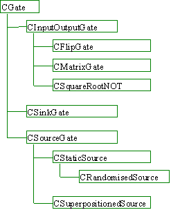
Figure 15
The base class for gates is the class CGate which provides a default implementation. It provides a number of methods that can perform the tasks listed below. Derived gates are able to override the implementation of any of these functions.
From CGate we then derive three more class - CInputOutputGate, CSinkGate and CSourceGate. CInputOutputGate provides a default implementation for gates with more than one input and output pin. (Remember from the background section that quantum gates must have an equal number of input and output gates). From CInputOutputGate two gates were derived for test purposes - CFlipGate and CSquareRootNOT. The latter performs the square root of not function on a single input bit, the former performs the function on one of its two input pins only if its other input pin has the value 1.
CSinkGate provides an implementation for sinks. Initially designed to cater for any number of input pins I later revised this to allow only one input pin in order to ease the implementation of certain simulator methods. CSourceGate allows data to enter the system. It’s derivation, CStaticSource exposes an output bit whose value is set at creation at 0 or 1. CRandomisedSource exposes an output bit whose value is randomly set at creation at 0 or 1.
The implementation of CSuperpositionedSource was later removed. The gate is functionally equivalent to a CStaticSource followed by a square root of not gate, i.e. the output is an equal superposition of 0 and 1. Again, allowing for such a ‘special’ gate created technical difficulties in other areas of the program. It was introduced due to an error in my thinking (see the later section entitled Original Design Error) where I thought that such a gate would greatly reduce the resources required by the simulation. Once the error was recognised I decided that the CSuperpositionedSource added little to the simulation while making the code less understandable and harder to maintain.
The class hierarchy for pins is shown below.
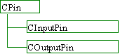
Figure 16
The abstract base pin class, CPin, provides the following default functionality.
From CPin we derive CInputPin and COutputPin. These classes simply specify the direction of the pin. The only purpose of having a direction on a pin is to ensure that we do not attempt to connect the output of two gates together. The pin classes hold the state information for connections and do not actually perform any work.
The ‘Simple’ Simulation Algorithm
Matrices For Gates
It was noted in the background section above that complex matrices can represent gates and that a complex vector can represent the state of the quantum system. The simulation of a gate in the system is then a tensor matrix operation on the state vector.
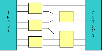
Before describing the simulation algorithm I shall explain an error that I made in my original design. I originally believed that each wire in a quantum circuit would require a separate quantum bit to simulate it. For example, I believed that the circuit shown in Figure 17 would require 17 quantum bits to simulate.
The following is a transcript from my log book entries for the 2nd to the 4th March 1997.
The original plan was proving hard to develop as I was not sure of the exact formulae for mapping the state to the system at one step in the simulation to the next state. So I did some research (mainly using P W Shor’s paper) and came up with a few new ideas and proofs.
Consider the following circuit.
We can then make the computation sequential (from point number 4, above)
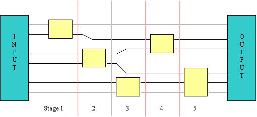
Figure 18
Important Deduction
At the end of each stage there are a constant number of bits, the number being equal to the number of input bits to the circuit. Therefore we can model the circuit with just 2n complex numbers, where n is the number of input bits. Therefore the computation time is now exponential in the size of the input, not in the size of the circuit as I had first thought. An exponential gain!
I have implemented a simulation algorithm based on the above deductions. A simulation of a circuit with 20 input bits and 40 gates required just 180 seconds. Such a simulation would not have been possible with the original design (it would have required 260 steps and 264 bytes of memory).
Out of the four points listed above the first three follow easily from a variety of quantum texts. It was this that led to the reduction in the memory requirements and steps required in the simulation. Point number four led to enough simplifications to develop the simulation algorithm – I simply needed to iterate the simulation looking at each gate turn. Previously I was unsure as to whether the simulation of a set of parallel gates could be performed in this manner or whether I had to perform some special computational tasks. Each gate can now be considered to act on a set of bits.
In hindsight, all the above points are implicit at the very least in a number of research papers. It took me a long time to recognise some of these points because I was unable to follow much of the complex terminology used in these very mathematical research papers.
It was the above reductions that led to the scrapping of ‘Quantum Bit Saving’ and superpositioned inputs. If the simulation needed to be exponential in the size of the circuit then each bit saving would have halved the simulation time and workspace – an exponential performance increase in the saving. However, with the simulation being exponential in the size of the inputs such idea would have only lead to a linear increase in the size of the saving. Thus saving one gate in a one hundred-gate circuit would only reduce the processing time by 1% and have had no effect on the size of workspace required.
Single Gate Simulation Algorithm
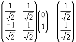
The simulation of a gate can be carried out by the multiplication of a gate’s matrix on its input amplitudes. Thus the square root of not gate acting on a 100% probability of its input being one results in the following computation.
The circuit is visualised in Figure 19.
What happens when there is more than one bit in the circuit? In Figure 20 we see that the second bit in the circuit must retain its value at the end of the simulation of the first bit.
The state vector for the entire circuit is initially ![]() , where the first element in the vector relates to the amplitude of observing |00>, the second to |01>, etc. We can see that this input vector must map to
, where the first element in the vector relates to the amplitude of observing |00>, the second to |01>, etc. We can see that this input vector must map to ![]() , i.e. there is no possibility of observing the second bit with a value of anything other than |1>, and there is an equal probability of observing the lower bit as |0> or |1>. The process to use is to apply the matrix for the square root of not gate to each possible value that may be observed in the rest of the circuit. We see that the second input may be |0> and then apply the square root of not gate. We then consider that the value of the second bit may be |1> and apply the matrix again. In the above example, this is equivalent to using the operation shown below.
, i.e. there is no possibility of observing the second bit with a value of anything other than |1>, and there is an equal probability of observing the lower bit as |0> or |1>. The process to use is to apply the matrix for the square root of not gate to each possible value that may be observed in the rest of the circuit. We see that the second input may be |0> and then apply the square root of not gate. We then consider that the value of the second bit may be |1> and apply the matrix again. In the above example, this is equivalent to using the operation shown below.
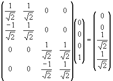
The idea had to be extended to cope with any number of bits in the circuit and any number of bits in the gate being processed.
‘Funny Counting’
The size of the intermediate matrix in the above matrix is 2n x 2n, where n is the number of input bits in the circuit. Obviously this matrix would be too big to generate for any reasonable size of inputs. Therefore it was decided to perform the smaller individual matrix operations on a selection of the input vector as opposed to attempting to perform one, large matrix multiplication.
Consider an n-gate system. A vector of length 2n represents the system, which means that we can access individual elements in the vector via an index that is an n bit number. Imagine attempting to simulate a two-bit gate acting on the first two bits of such a system. If we were to denote the bits that the gate operates on by the letter ‘G’ and the rest of the bits by the letter ‘R’, then the map of the bits of the index would look like this.
RRR…RRR GG
In order to simulate the gate we need to apply the gate matrix to every possible combination of the other bits in the system. In the current example that involves iterating through the bits denoted by R. The project source code and other areas of this document denote the value of R at some point in the simulation the ‘base amplitude’ of that point. The bits denoted by G are iterated over to provide the four input elements for the multiplication by the gate’s matrix. Thus every element in the [exponential] state vector that represents the system must be accessed to simulate every gate. The mapping for an arbitrary R is shown below.
|
State vector element |
Becomes position |
|
RRR…RRR 00 |
Input vector element 1 |
|
RRR…RRR 01 |
Input vector element 2 |
|
RRR…RRR 10 |
Input vector element 3 |
|
RRR…RRR 11 |
Input vector element 4 |
The mapping for the entire simulation of the example gate is given below.
|
Input Vector |
Multiplication 1 |
Multiplication 2 |
… |
Multiplication 2n-2 |
|
Element 1 |
000…000 00 |
000…001 00 |
… |
111…111 00 |
|
Element 2 |
000…000 01 |
000…001 01 |
… |
111…111 01 |
|
Element 3 |
000…000 10 |
000…001 10 |
… |
111…111 10 |
|
Element 4 |
000…000 11 |
000…001 10 |
… |
111…111 11 |
Now consider that we wish to simulate a gate in an 8-bit system that acts on the input bits five and two. Obviously, as with gates in classical systems the order of the input connections is important. The mapping for the simulation of this gate is shown below. Notice that the iteration over the bits of the gate is carried out in the correct order.
|
Input Vector |
Multiplication 1 |
Multiplication 2 |
… |
Multiplication 28-2 |
|
Element 1 |
00 0 00 0 00 |
00 0 00 0 01 |
… |
11 0 11 0 11 |
|
Element 2 |
00 1 00 0 00 |
00 1 00 0 01 |
… |
11 1 11 0 11 |
|
Element 3 |
00 0 00 1 00 |
00 0 00 1 01 |
… |
11 0 11 1 11 |
|
Element 4 |
00 1 00 1 00 |
00 1 00 1 01 |
… |
11 1 11 1 11 |
It is easy to extend this algorithm to cope with bits of an arbitrary size.
I dubbed this task ‘funny counting’ as the iteration of counter that is used to index the state vector increments in a funny order. Pseudo-code to implement this algorithm is shown in the next section.
Simulation Algorithm
The above ideas can be used to implement a simulation algorithm. The pseudo-code for this algorithm is shown below.
OrderGates()
For each gate in the system.
For BaseAmplitude = 0 .. 2n-1
If BaseAmplitude does not have a bit set which our gate uses
For GateAmplitude = 0 .. 2bits in gate-1
InputVector[ GateAmplitude ] =
SystemState[ BaseAmplitude $ GateAmplitude ]
End for
OutputVector = GateMatrix * InputVector
For GateAmplitude = 0 .. 2bits in gate-1
SystemState[ BaseAmplitude $ GateAmpltidue ] =
OutputVector[ GateAmplitude ]
End for
End if
End for
End for
Care must be taken to ensure that the gates are processed in dependency order. If there are two gates in the system such that the second gate depends on the output of the first gate then we must ensure that the first gate is simulated before the second gate. An ordering function is applied to the list of gates in the circuit before the simulation commences to ensure that this condition is not broken.
The operation $ is used to combine the iterations over the base amplitude and the gate amplitude. Bit x in the gate amplitude is mapped to bit y in the base amplitude, where y is the circuit bit which input pin x works on.
A number of basic tests on the values output by the simulator was performed at this stage. See the Testing section later for an overview of the testing algorithms, though note that not all of the tests listed in that section were implemented at this stage.
After the initial implementation of the simulator was finished I decided that the next most important step was to implement the ability to read in files describing the circuit. Since my original specification of the project it had become apparent that researchers in the field of quantum computation tended to describe their circuits mathematically. Further, the matrices of certain gates with these circuits sometimes had values that were determined by mathematical equations depending upon their position in the circuit. Many circuits also exhibited a recursive quality.
Bearing this in mind I decided to scrap the original plans for the structure of the input file. The example structure as shown in the section entitled ‘The Simulator’s Final Design’ did not allow mathematical equations. To extend the system to cope with equations would have involved writing a parser. To allow recursion would have involved designing an input file format that would be programmable.
I started research in to the amount of work involved in developing a programmable input file format. I estimated that designing and implementing a format of sufficient quality would take about two weeks of full time programming. Whilst undertaking the research I realised that many of the formulae and constructs in quantum computing texts could be handled be a lazy evaluation technique. As such they were ideal for representing in a functional programming language. I decided that the ideal situation occur if I could find a publicly available C or C++ source-code implementation of a functional programming language. The program could then be integrated within my project. Some further research continued and I managed to find HUGS, a C implementation of the functional language Haskell.
After investigating the source code and capabilities of HUGS I decided that the best way of integrating the program with my own was to leave HUGS as an external program which was called to process circuits. This saved reworking the program to make it compatible with the simulator. However in order to maintain the maximum precision while simulating circuits I modified HUGS to make sure that it used double-precision floating-point numbers throughout.
I decided that the output from HUGS should be a bare sequence of numbers. This minimised the complexity of the parser that I had to build in to the simulator.
Finding HUGS was a stroke of luck. I estimate that it took me about a week to learn HUGS and integrate it within the simulator. The alternative would have been to implement some language myself, which would have been far less powerful and not compatible with the constructs of the major functional languages. The alternative would have also taken at least an extra week of work. The extra time that I spent researching the area of input files certainly paid off and saved me attempting to re-invent the wheel.
In order to capture the output from HUGS in to my application I developed a parser in the simulator was made to take tuples in the form (number of bits in the circuit, initial input value, ordered list of gates). The definition of a gate was (ordered list of bits to act upon, ordered list of complex numbers in the gate matrix). For example, the square root of not gate acting on a single bit circuit with an initial value of 0 would be (1, 0, [ ( [0], [ 0.707, -0.707, 0.707, 0.707 ] ) ] ).
I then made a set of Haskell libraries for HUGS to output this raw data. There are two Haskell files – gates.hs defines the gates used in a circuit, while circuit.hs defines the circuits. The square root of not gate, for instance, requires the following code in gates.hs.
type Gate = ([Int], [Complex Double])
oneOverRootTwo :: Complex Double
oneOverRootTwo = 2**(-0.5) :+ 0
--------------------------------------------------------------------------
-- Matrices
sqrtNotMatrix ::[ Complex Double ]
sqrtNotMatrix = [ oneOverRootTwo, -oneOverRootTwo, oneOverRootTwo, oneOverRootTwo ]
--------------------------------------------------------------------------
-- sqrtGate n, where n is the bit for the gate to act on
sqrtGate :: Int -> Gate
sqrtGate n = ([n], sqrtNotMatrix)
We can easily extend this code to allow circuits made up of square root of not gates. For instance by using the following code.
-- sqrtGates [n]. Constructs a column of sqrtNot gates, where
-- [n] gives the bits to act on
sqrtGates :: [Int] -> [Gate]
sqrtGates [] = []
sqrtGates (b:bs) = (sqrtGate b) : sqrtGates bs
And in circuit.hs we have the following code.
type Circuit = ( Int, Int, [Gate] )
-- test circuit
notTestCircuit :: Int -> Int -> Circuit
notTestCircuit (n+1) i = (n+1, i, (sqrtGates [0..n]) ++ (sqrtGates [0..n]) )
A 10-bit circuit to invert the number 53, for example, would be created by typing in the command
notTestCircuit 10 53. We could simulate this circuit opening the file circuit.hs from within the simulator. After this, the user would select the option ‘Start Simulation’. This, in turn, causes the simulator to ask the user for the Haskell command to execute. HUGS is then invoked, the command is piped in to it and its output is captured. The parser within the simulation then reads and parses the HUGS output and creates a circuit from the description.Optimised Algorithms
Summary
To summarise, optimisation of the simulator by a variety of methods and algorithms has lead to a hundred-fold increase in execution speeds and a ten-fold decrease in memory requirements over my original simulator code in certain situations.
The benchmark machine for my tests was a Cyrix P166+ machine with 32Mb of memory. The Cyrix processors are considered to have a better integer performance than an equivalent Intel processor but worse floating point performance.
Some of the results have proved surprising. I had expected that it would be possible to simulate concurrent gates concurrently. Alas the laws of quantum mechanics had something to say about that idea! I had to rewrite my threads to use concurrency in other areas of simulation. I had expected my cache-hit increasing ‘complex’ algorithm to reduce execution times for all reasonably sized circuits. However it only produces increases the performance in low memory situations (i.e. large simulations). I had also expected that multi-threading would not lead to any increase in performance on a single processor machine. However there is a remarkable increase in performance using multiple threads when the memory is low.
Profiling
The first gains in execution time came from using profilers on simulations in order to spot areas of the simulation that were occupying the most processor time, and thus which areas I should concentrate on optimising. The results from the first profile showed that the simulator was spending approximately 85% of its time creating and destroying vectors and less than 10% of its performing the essential matrix calculations.
This inefficiency was due to returning vectors on the stack. Consider the following code.
Main( )
{
Matrix m = ...;
Vector v = ...
Vector r;
r = m.Multiply( v );
}
// Method to multiply a matrix by a vector
Vector Matrix::Multiply( Vector &v )
{
Vector r;
// Multiply performed here
return r;
}
C++ compilers in translate this to the following sequence of instruction. Extra code generated by the compiler is highlighted.
Main( )
{
Matrix m = ...;
Vector v = ...
Create vector v
Vector r;
Create vector r
r = m.Multiply( v );
perform the multiply, result returned on the stack in vector ‘temp’
destroy contents of ‘r’
copy ‘temp’ in to ‘r’
destroy contents of ‘temp’
}
// Method to multiply a matrix by a vector
Vector Matrix::Multiply( Vector &v )
{
Vector r;
create vector r
// Multiply performed here
return r;
create vector ‘temp’
copy r in to ‘temp’
destroy ‘r’
}
Now consider what happens if we pass the v in to the function by reference.
Main( )
{
Matrix m = ...;
Vector v = ...
Create vector v
Vector r;
Create vector r
m.Multiply( v, r );
perform the multiply, result returned on the stack in vector ‘r’
}
// Method to multiply a matrix by a vector, returning the result in r
Matrix::Multiply( Vector &v, Vector &r )
{
// Multiply performed here. Results placed in ‘r’
return ;
}
The second code segment above removes the need for the temporary variables and copies. It saves two vector creations, two vector copies and three vector destructions. As the multiplication operations performed by the simulation are generally quite small this results in a substantial increase in the efficiency of the simulation algorithm. Further efficiencies were gained by moving vector creation for temporary vectors outside of the inner loops of the simulation.
Optimisation based on the results of the profiler have allowed me reverse the original profile results. Now, the system spends less than 5% of its time creating and destroying objects and over 85% of its time performing the matrix calculations, resulting in an increase of performance by a factor of ten.
localising memory accesses (Cache-Hit Increasing & Page-fault decreasing)
Idea
In the description of the simple simulation algorithm above it was shown that the simulation of every gate in the system required access to every element in the state vector. As the state vector is likely to be many megabytes in length the system will not be able to cache the data in the processor cache. Further, if the size of the state vector exceeds the physical memory available to the simulation then the system will have to continuously page the state vector in and out of memory. This continuous paging will result in a severe degradation in system performance.
The solution to the above problems is to localise the memory access as much as possible. In the simple simulation the loop which iterates over the gates is the outermost loop. In the ‘complex’ memory localising method we move the gate loop inwards.
An recap of the simulation code is shown below.
For each gate in the system.
For BaseAmplitude = 0 .. 2n-1
If BaseAmplitude does not have a bit set which our gate uses
Perform calculations….
End if
End for
End for
Care must be taken reordering the loops to ensure that we preserve the ordering of dependent calculations within the simulation. Moving the gate-processing loop inside the loop that iterates over the amplitudes would not necessarily preserve this ordering. To preserve the order we need to perform some analysis on the dependencies within the simulation.
Suppose that we have two sequential gates as shown in Figure 21. The input of the second gate is entirely dependent on the output of the first gate. In this case it is possible to move the gate-processing loop inwards provided that we still ensure that the calculations of the first gate occur before those of the first gate.
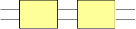
Now imagine that we have two parallel gates as shown in Figure 22. Remember that the operation of a single gate affects the state of the entire system, not just the state of the bit(s) that it is working on. Because of this it is not possible to move the gate-processing loop inwards without some extra work to ensure that the correct ordering of calculations is preserved. As was mentioned in the description of the simple simulation algorithm, it does not matter which of the two gates is simulated first. However it does matter that the actions of the gates appear to be atomic. For instance, it would be incorrect if we allowed the first gate to perform a partial computation, use the resultant state as the input to the second gate and then allowed the first gate to use the result from the second gate to complete its calculations. (This is why my first attempt at a multi-threaded algorithm, described later, failed.)
Imagine the situation where the first gate is connected to bits 0 and 1 of the circuit and the second gate is connected to bits 2 and 3. Also imagine that we have (arbitrarily) decided to simulate the first gate before the second one. The trace of the accesses to the state vector is shown below. The simulation of each gate in this circuit requires two matrix multiplies, each involving a vector with two elements.
|
Matrix Multiply |
First Gate |
Second Gate |
|
1 |
Element 00 |
Element 00 |
|
1 |
Element 01 |
Element 10 |
|
2 |
Element 10 |
Element 01 |
|
2 |
Element 11 |
Element 11 |
As you can see, the accesses of the matrix multiplies of the second gate are dependent upon the results from both of the outputs of the matrix multiplies of the first gate.
Now imagine if we extended the circuit to operate on three bits, as Figure 23, where the third bit in the circuit plays no part in the area of the simulation that we are looking at.
The simulation of each gate now requires four matrix multiplies. The traces of accesses to the state vector for the simulation of this system would be as follows.
|
Matrix Multiply |
First Gate |
Second Gate |
|
1 |
Element 000 |
Element 000 |
|
1 |
Element 001 |
Element 010 |
|
2 |
Element 010 |
Element 001 |
|
2 |
Element 011 |
Element 011 |
|
3 |
Element 100 |
Element 100 |
|
3 |
Element 101 |
Element 110 |
|
4 |
Element 110 |
Element 101 |
|
4 |
Element 111 |
Element 111 |
As you can see, again the first two matrix multiplies of the second gate are dependent upon the output of the first two multiplies of the second gate. Notice, however, that they are not dependent upon the results of the third and fourth matrix multiplies of the first gate. Thus we could schedule the first and second multiplies of the second gate to occur before the third and fourth multiplies of the first gate.
If we were to schedule the first matrix operation of the second gate before the second operation of the first gate then we would localise the memory accesses. The first four matrix multiplies would access the only four elements of the state vector only. Previously, when we had to compute the entirety of the first gate before the second gate, the first four matrix operations required access to all eight elements of the state vector.
The above example can be turned in to a generic algorithm. If we consider a group of gates that act on an arbitrary number of bits, then we must perform the iteration of the ‘Base Amplitude’ over the bits that these gates act on in some defined order. The iteration over the rest of the bits in the circuit can be performed any order. The algorithm for simulating a group of gates in the circuit in order to localise memory accesses is as follows.
For BaseAmplitude = 0 .. 2n-1
If BaseAmplitude does not have a bit set which our group of gates use
For each gate in the group
For GroupAmplitude = 0..2n-1
If GroupAmplitude has only bits set which the rest of the group uses
Perform calculations….
End if
End for
End for
End if
End for
Notice that the expense of moving in the gate-processing loop is that we have to add another loop inside of it. This new innermost loop appears to be exponential and it would seem that the cost of localising memory accesses is to raise the processing requirements from 2n to (2n)2. However this is not the case. The innermost if statement ensures that the calculations for each gate are still performed the same number of times for each gate. Further, by including some clever bit masking and setting logic we can ensure that the innermost if statement is only called c*2n times, where c << 2n. (Effectively we reason that a failure on an if statement is caused by a single bit being set when it should not be and we can use this to increment the for counters in non-linear jumps). Despite these steps the localisation does require extra control overheads than the simple algorithm. A comparison of the two algorithms is shown later.
Grouping Gates
Modern microprocessors have a level-1 cache of around 16Kb and a level-2 cache of around 256Kb. In order to make the most of these caches we must ensure that the localisation takes in to account their sizes. For that reason the entire set of computations in a complex simulation are partitioned in to groups that work on small areas of around 256Kb. These groups are then partitioned further in to sub-groups that work in areas of around 16Kb.
The class CGateGroup was designed in order to represent a set of gates. The class has the following functionality.
The class CQList was created to help in the implementation of CGateGroup. This class implements a polymorphic list that can order its elements, subject to a partial or total ordering imposed on its elements.
Three methods in the class CMetaverse are used to the partitioning and simulation.
The method PartitionGroup deserves a fuller account. Given a set of gates it produces a list of groups. The groups are ordered in to computation order – that is if a group X precedes group Y then none of the inputs of the gates of X depend upon the outputs of the gates of Y.
Suppose for instance that we wished to partition a circuit in to groups with a localisation size of 512 bytes. 512 bytes equals 32 complex numbers at 16 bytes per complex number. In order to make sure that we localise access to the state vector to 32 (i.e. 25) elements at a time we must limit the number of bits that the gates within each group uses to 5.
The first thing to do is to order the input list of gates to partition in to a simulation order which attempts to keep related gates as close together as possible. For instance suppose that we have four gates A, B, C and D, and the input of B depends on the output of A (A < B, or A "precedes" B), B < C and A < D. The dependency graph for this is shown in Figure 24. The ordering method will then output the list {A, B, C, D} or {A, D, B, C}. However it would not output {A, B, D, C}, even though this list preserves the partial ordering, as the related gates B and C are not as close together as possible. (Having said that, in order to reduce the ordering time the algorithm is a heuristic and is not guaranteed to produce the correct output all of the time).
Now we attempt to group the ordered list. The first gate in our imaginary list to partition is as in Figure 25. We now wish to add to this group the maximum number of gates subject to the ordering and size constraints. This gate already uses 2 bits so we have at most 3 more bits to play with. By the ordering property above the next gate in the list will be gate B. This uses the same bits as gate A so the localisation is not going to be affected by adding this gate to the group. Therefore we add it. Now we come to gate C – this uses three pins, none of which are in common with the other two gates. We add this gate to the group, leaving us no more bits to play with. Gate D uses the same bits as the other gates, and so it is added. Gates E and F cannot be added without exceeding our quota of bits and so they are left to be placed in the next group.
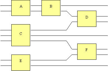
As you can see the partitioning algorithm is very dependent upon the partial ordering method of the CQList.
Multiple Threads
Initial Algorithm
The cache hit increasing ‘complex’ algorithm orders the circuit to be evaluated in to a set of non-overlapping groups. Dependency information is kept on the groups and one can consider the whole to be analogous to a series of transactions to be executed in a database. It was my original intention that separate threads should calculate concurrent groups. This was part of the reason for creating the complex algorithm in the first place.
I designed and implemented an algorithm to perform the above task and the algorithm worked exactly as intended. Unfortunately, using the algorithm resulted in a sizeable fraction of the automatic tests returning incorrect results. I investigated the matter and determined that the cause of the problem lay in the nature of quantum circuits. I believe it was a reasonable thought that two concurrent gates could be simulated concurrently. In classical circuit the output of the two gates would not have interfered with each other. However in a quantum circuit the two gates do interfere. Another way of describing the state of two or more superpositioned bits is calling them ‘entangled’, i.e. affecting one of the bits produces an effect on the other. Here we see interference working, and this is why my original algorithm failed.
Final Algorithm
The above algorithm sought to introduce concurrency in the processing of gates. There was another plan for introducing many threads that I had also planned for, and that was to introduce concurrency in the sheer number of matrix multiplies required to simulate a gate. The simulation of a two bit gate in an n bit circuit requires 2n-2 non-overlapping matrix multiplies, and so there is plenty of scope for parallelisation.
Each matrix multiplication is likely to be small and the cost of thread synchronisation would make it inefficient to allocate each multiplication to a separate thread. Further, the non-linear ordering of the matrix operations make it hard to divide the multiplications in to groups without decreasing efficiency. However the cache hit increasing algorithm groups many gates together. The matrices multiplies involved in simulating a group of gates are much less inefficient to thread and it is these which are allocated to separate threads. In the example shown in the description of the memory localising algorithm above, and recapped below, the first two matrix multiplies of the first and second gates would go to one thread, the last two to another, as theses sets of operations do not interfere with each other.
|
Matrix Multiply |
First Gate |
Second Gate |
Thread |
|
1 |
Element 000 |
Element 000 |
1 |
|
1 |
Element 001 |
Element 010 |
1 |
|
2 |
Element 010 |
Element 001 |
1 |
|
2 |
Element 011 |
Element 011 |
1 |
|
3 |
Element 100 |
Element 100 |
2 |
|
3 |
Element 101 |
Element 110 |
2 |
|
4 |
Element 110 |
Element 101 |
2 |
|
4 |
Element 111 |
Element 111 |
2 |
The task for controlling the threads is called CCalculationThreads. The complex algorithm creates one when it has determined that the user requires more than one thread in the simulation. A parameter passed in the construction of a CCalculationThreads object gives the number of threads to create. The pseudo-code for the algorithm is summarised below.
New CCalculationThreads( NumberOfThreads, ThreadPriority )
…
for each sub-group
for each base amplitude
queue amplitude to process the gates for
end for
wait for queue to empty
end for
The pseudo-code for an algorithm that queues amplitudes is listed below.
wait for free slot to queue amplitude
add the amplitude to the queue
signal data in queue to process
The pseudo-code for an algorithm that processes queued amplitudes is listed below.
wait for data in queue to process
calculate gates for this amplitude
signal free slot in amplitude queue
Semaphore objects are used to handle the queue lengths. A mutex object controls access to the CCalculationThreads object. Each gate calculation requires two vectors to store temporary data for the calculation. This temporary data is created at the time of the creation of the CCalculationThreads object as the continuous creation of temporary vectors would result in a large amount of time being spent creating and destroying objects.
Result
A trace of the percentage of processor time occupied by each thread in a quad threaded simulation is shown in Figure 26 below. There are two extra threads. The ‘Main Thread’ is the thread that is responsible for starting the simulation. It starts up a separate thread, the ‘controller’ for the purposes of running and controlling the simulation. After this second thread has started the first thread handles the simulation progress dialogue box. Hence the thread performs a large amount of initial work as the dialogue box is drawn. The controller thread then starts to prepare the simulation. It is responsible for initialising the vectors for the simulation, starting off the calculation threads and then queuing the amplitudes to process. You can see it peak at the start as it initialises, then occasionally require the processor to send data to the calculation threads throughout the simulation. The four other threads are used to perform the calculations. These oscillate around 25% processor time, as one would expect.
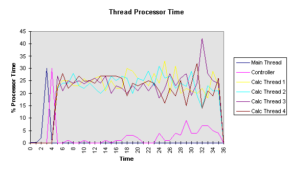
The slightly erratic behaviour towards the end of the graph is due to the uneven partitioning of the gates to be processed. The partitioning of the complex algorithm breaks this 18 bit circuit in to effectively non-overlapping groups of 7, 7 and 4 bits. Each of these groups is simulated separately. The 7 bit groups have 14 gates and the 4-bit group has 8 gates. The algorithm allocates work to each thread in sizes which are proportional to 2n, where n is the number of gates in the group. Thus, towards the end of the simulation smaller parcels of work are being handed out. The consequence is that the controlling thread has to perform proportionally more work in comparison to the other threads when with smaller groups have to be simulated. Further, the algorithm for allocating work to the threads does not attempt to divide the work equally amongst the threads. If a thread can complete its allocated task before the controlling thread allocates the next task then it is possible that it may get allocated the next task, and the one after, and so on. One thread, therefore, may perform all of the work. This is why one thread above has managed to peak at about 42% of processor time towards the end of the simulation.
I do not consider this to be a bug in the code as I have yet to see any adverse side effects from the above behaviour. Indeed, one could argue that the above behaviour has distinct benefits in a multiprocessor environment as we would like as much work as possible to be performed by one processor. This would reduce the number of cache misses that would occur if the work were switched to another processor. Also, the amount of work that needs to be performed by the simulation is always the same, as is the amount of thread synchronisation required and both are independent of the size of the groups.
Sparse Vectors
Sparse vectors were implemented by reorganising the original vector implementation. A new class, CBaseComplexVector, was added to provide a default implementation for vectors. It provides default methods for setting and returning the length of vectors and performing mathematical operations on the vector and its elements. It expects derived classes to provide methods for setting and returning the individual elements of the vector. The class CComplexVector now represents statically allocated vectors – the old name was kept to preserve compatibility. CSparseComplexVector was added to represent sparse vectors. The updated class hierarchy for vectors is shown in Figure 27.
My sparse vector implementation is quite simple and works by dividing the vector that it is to represent in to an array of sections of a pre-determined size. Each of these sections is in itself a small static vector and is represented by a CComplexVector. Initially empty vectors represent these sections and thus require a minimal amount of memory. An attempt to read from an empty vector returns the complex value of 0. An attempt to write a value 0 to an empty vector is ignored. An attempt to write a value of anything other than 0 to an empty vector results in the vector being allocated and the corresponding element being set. Reading or writing to a non-empty vector causes the corresponding element to be returned or set, respectively.
At the moment the vector does not automatically shrink itself. The code to achieve this is relatively straightforward and has already been implemented, though it has not been enabled. My purpose in using sparse vectors was to reduce the maximum memory requirements of the application, not the average requirements.
The section size is determined at compile time. Smaller section sizes result in a greater memory overhead and generally a higher execution time though it could reduce the amount of memory required to represent the vector. A comparison of the amount of memory required to simulate a quantum Fourier transform is shown below.
Comparison Of Simple And Complex Simulation Algorithms
The run time of the Quantum Fourier Transform is shown in Figure 28 for the benchmark system when there was plenty of memory available for the simulation. The difference between the simple, complex single-threaded and complex multi-threaded algorithms does not very greatly under these conditions. The complex single-threaded algorithm is about 5% slower than the simple algorithm and the complex multi-threaded algorithm is around 10% slower at its worst. As these variations are small in comparison to the exponential time of the simulation separate graphs for their performances are not shown.
The performance is as expected for the Fourier transform at around O( n22n ), where n is the number of input bits to the circuit. Thus adding an extra bit to the transform multiplies the processor work required by a factor of around 2.2. The workspace requires 2n complex numbers at 16 bytes per complex number.
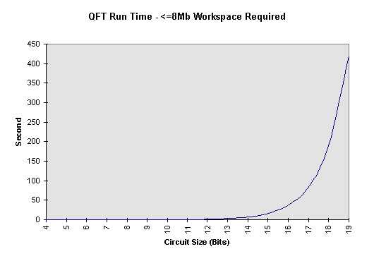
The situation becomes more interesting at the memory requirements of the simulation start to exceed the physical memory available. The benchmark machine has a total of 32Mb of physical memory. The Windows NT operating likes to keep around 16Mb for its kernel, a disk cache and a set load loaded libraries. Thus there is only 16Mb left for the simulator and its workspace. Leaving a megabyte for the simulator code means that the entire simulation workspace cannot entirely fit in to memory and a small amount of paging is inevitable.
Figure 29 shows the timings for simple, complex single-threaded and complex multi-threaded simulations on a 20 bit Fourier transform. The complex algorithms have to perform more work as they have to order the calculations of the gates. In order for the complex algorithms to be quicker the processor time saved by the reductions in the number of cache misses and page faults has to compensate for this loss. Here the amount of paging is not high enough to allow the complex single threaded algorithm to regain the processor time required for the ordering. However the complex multi-threaded algorithm can regain this ‘lost’ processing time.
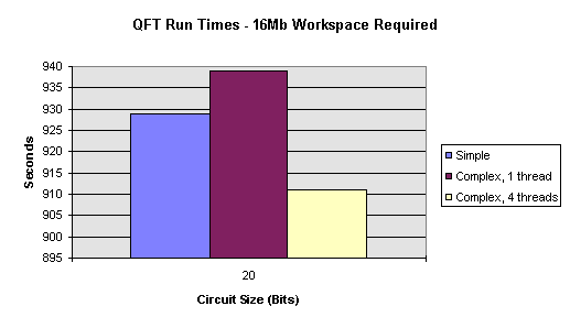
I was not expecting to see any gains using multiple threads on a single processor machine. In fact I was expecting a five to ten percent performance degradation as the multiple threads require extra controlling. Locks, semaphores and mutex’s are all used within the simulator to control access to resources, queue requests for calculations and queue any free threads. I was therefore surprised to see the above result and sought an explanation.
The reason for the extra speed comes stems from NT switching threads when one is blocked after causing a page fault. Imagine a thread that requires access to a memory location that swapped out at that time. NT will queue a request for the required memory page. However this will take upwards of 15ms to arrive from the hard disk. When running a single threaded simulation the operating system has no choice but to block waiting for the page to arrive. However in a multi-threaded simulation it is possible that some other thread does not require a swapped out page and is able to run. If so NT can switch tasks to that thread, thereby saving the 15ms which, on modern microprocessors, equates to several million processor instructions.
The run times become even more interesting when the amount of memory required greatly exceeds the amount of physical memory available. The simple simulation algorithm makes no attempt to localise memory accesses in order to reduce the number of page faults. Thus the simulation of each gate requires access to all of the complex numbers in the simulation workspace. For a 21 bit Fourier transform, timings for which are shown in Figure 30, the simulator forces the reading and writing of 32Mb of data for each of the 273 gates. That is approximately 8.5 Gb reading and writing, and would take a modern PC hard disk approximately an hour if the accesses were sequential. Unfortunately, the memory access is not sequential (see ‘Funny Counting’, above) and so the time spent waiting for the hard disk is far greater than this.
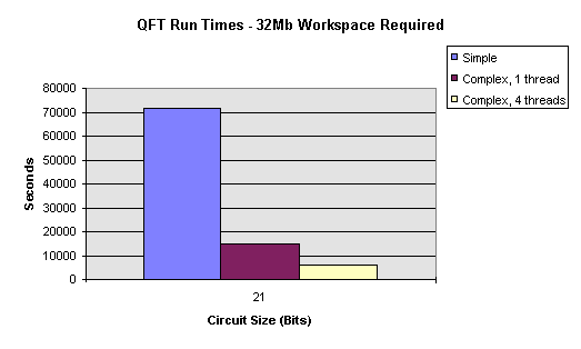
The amount of pure processor time required for the simulation of the 21 bit Fourier transform should be 2.2 times more than a 20 bit transform, and thus around 2,000 seconds. The simple simulation requires around 72,000 seconds, i.e. the system spends thirty-five seconds waiting for the hard disk for every one second it spends calculating the circuit’s outputs. The single-threaded complex simulation is far more efficient at around 15,000 seconds. The quad-threaded complex simulation requires a mere 6,000 seconds in comparison.
The conclusion is that the simple algorithm is more efficient when the system’s physical memory requirements are sufficiently large to fully satisfy the workspace required for a simulation. The extra overheads of the ordering of the complex algorithm and the communication and synchronisation of the threaded algorithms means that the two algorithms are around five and ten percent slower, respectively. However the simple algorithm is unable to scale to situations where the memory requirements of the simulation are not met by the system. The complex algorithms have been designed to scale better and perform well. The multi-threaded algorithm performs excellently and exceeds my original expectations.
Comparison Of Sparse And Static Vectors
The comparisons below in Figure 31 show the difference between the observed maximum memory requirements of the simulator when performing a Quantum factorisation. It should be noted that the amount of space required by the sparse vector depends to some degree upon the random number that the Quantum factorisation algorithm uses, and can extend to as much as twice the values recorded here. I have chosen use this particular circuit to demonstrate the algorithm as it a ‘real world’ application. The Quantum Fourier transform by itself, as used in the comparisons above, requires the sparse vectors to use maximum amount of memory at some time, and so does not offer any opportunity for gains. The sizes of the sparse vector section used in these tests were 128 elements.
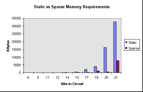
Figure 31
As you can see signification gains can be achieved by using sparse vectors. This is, however, accompanied by a 30% slowdown in execution times.
Comparison of Size of Sparse Vector Sections
As you can see in Figure 32 changing the size of the sections in the sparse vectors does not greatly make a difference to the maximum amount of memory that is required by a simulation. The tests were performed on various sizes of quantum factorisations that were run with a set ‘random’ number and number to factorise. A smaller section size will offer a greater memory reductions where the complex values that represent the system’s state are sharply defined and widely spaced. A larger section size offers less computational overhead. The 128-element section size provides good compromise between these two ideals.
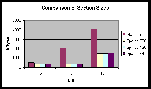
automated testing
The automated testing was designed to catch errors that may occur when making changes to the core simulation code or introducing new methods of simulating a circuit. At the core of the system are seven standard test circuits. They are listed below. Each circuit can be any size and is made up of a single, basic building block that is repeated throughout the circuit. The circuits were designed to produce a single definite output from a single input. They were designed to catch problems that were likely to occur whilst being easy to verify.
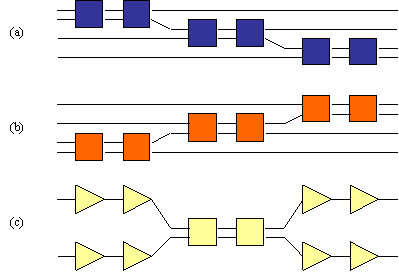
The first four tests were designed to highlight any problems in the basic creation of the circuits and the simulation of simple systems. The last three tests were designed to test the interactions between bits and catch problems that may come from attempting to order the calculations.
The automated tests selects a test circuit randomly, makes it a random size (up to user a specified maximum), chooses a random input, selects a random simulation algorithm (simple or complex), selects a random number of threads if the algorithm is complex and then randomly chooses between static and sparse vectors. The combined effect is to allow hundreds of millions of possible tests.
As the automated test algorithm knows which test it has created, and the inputs to that test, it is able to work out what the output should have been. Upon the test’s completion the output is compared to the ideal and the opportunity to stop the program is given to the user. The automated tests continue until the user intervenes.
I have not yet found a circuit that fails to simulate correctly after the simulator has passed a large number of these tests. Typically, major errors in the simulator implementation are revealed quite early by these tests. Minor problems, such as problems associated with accessing memory via C++ pointers, usually appear within a hundred tests or so. I will typically run 2,000 tests after changing the simulator code and periodically run 10,000 tests.
Internal Tests
The debug version of the simulator has over 200 testing points scattered throughout the code where pre-conditions, post-conditions and invariants are tested throughout execution. The application is very stable and has few known weaknesses. Exception handlers are used in the program so that an error in most parts of the program will be handled gracefully and not cause the entire application to crash.
Overall I would classify the project as a success. I have set out everything that I planned to achieve and in certain areas, such as the flexibility of the input file, I have exceeded my expectations.
There were a number of difficulties that arose along the way that could have been avoided. The two areas that I got the most wrong were the number of bits required to simulate a circuit and the inability to simulate concurrent gates concurrently. The first problem was due to a lack of proper understanding of the project (probably due to believing that I knew what was going on when in fact I didn’t!). The second problem was due to not researching the task properly and not thinking about the results. I certainly knew enough by that stage to avoid making that mistake.
There are a number of areas that I would like to improve with the current implementation. The user interface could do with a lot more planning. It has been put together in a manner which suggests a lack of forethought.
On the Haskell side error messages need to be improved, perhaps by integrating the simulator more fully with the Haskell interpreter. At the moment the simulator effectively knows nothing about the Haskell code which outputs the set of complex numbers. An error in the Haskell code is usually relayed to the user as "ERROR: Expected (", as opposed to a nicer "Error at line 53 in Circuit.hs, etc. etc."
On the simulator side more research should be done to determine which of the various algorithms produce the best results. Perhaps a heuristic could be used to suggest to the user which algorithm is likely to lead to the quickest simulation. My sparse vector implementation was an algorithm which was invented ‘off the cuff’. There has been a lot of published work in this area and proper research could considerable speed up the computation and / or reduce the memory overhead even further.
The areas where the simulator could be extended to are almost boundless. It may be nice to create some sort of graphical editing tool for creating circuits. The reason why I did not investigate this further was because the addition of a single gate affects the output of the entire system. Thus it is very hard to imagine anybody being able to create any useful quantum circuit by dropping circuits on to an editor and then connecting the pins. However as an education tool it could be invaluable. With some visualisation tool it could be used to demonstrate what is going on inside the quantum circuit.
A better way of visualising the amplitudes in the circuit would be nice. The main problem here is that the complex state of the system is inherently multi-dimensional. In fact the state at any given point is described by a point on a sphere in n-dimensional space, where n is the number of bits in the system. A program to visualise this space would be a large project in itself.
The ultimate quantum circuit simulator would be one that uses a quantum circuit to simulate other circuits, thereby reducing the exponential overheads. Such a goal, however, is a decade away at the very least.
Bibliography and References
There is much material on the WWW on the subjects of quantum computation, quantum cryptography and quantum information theory.
http://xxx.lanl.gov/archive/quant-ph - Quantum Physics archive at Los Alamos National Laboratory http://eve.physics.ox.ac.uk/Qchome.html - Quantum Computation and Cryptography Home Page at Oxford http://vesta.physics.ucla.edu/~smolin - John Smolin’s Quantum Information Page http://chemphys.weizmann.ac.il/~schmuel/comp/comp.html - Samuel L. Bernstein’s Tutorial on Quantum ComputationFor an excellent introduction to the Many Worlds theory I recommend the many-worlds-faq by Michael Clive Price, which is available on the world wide web.
A number of articles about quantum computing have appeared in popular scientific magazines. I recommend:
Julian Brown, A Quantum Revolution for Computing, New Scientist, 24 September 1994, pp. 21-24
D. Deutsch, Quantum computation, Physics World, June 1992.
Seth Lloyd, Quantum Mechanical Computers, Scientific American, October 1995, pp. 44-50.
http://www.economist.com/issue/28-09-96/st4046.html – The Economist, The Weirdest Computer of All.
P. Benioff (1980), The computer as a physical system: A microscopic quantum mechanical Hamiltonian model of computers as represented by Turing machines, J. Statist. Phys., 22, pp. 563-591.
P. Benioff (1982a), Quantum mechanical Hamiltonian models of Turing machines, J. Statist. Phys., 29, pp. 515-546.
P. Benioff (1982b), Quantum mechanical Hamiltonian models of Turing machines that dissipate no energy, Phys. Rev. Lett., 48, pp 1581-1585.
C. Bennet (1973), Logical reversibility of computation, IBM J. Res. Develop., 17, pp. 525-532.
C. Bennett, E. Bernstein, G. Brassard, U. Vazirani (1996) Strengths and Weaknesses of Quantum Computing, available from
http://xxx.lanl.gov/archive/quant-phE. Bernstein and U. Varirani (1993) Quantum Complexity Theory, Proceedings of the 25th Annual ACM symposium on Theory of Computing, 1993, 11-20
G. Brassard (1996), New trends in quantum computing, 13th Symposium on Theoretical Aspects of computer science, Grenoble, France, 22 - 24 February 1996.
D. Deutsch (1985), Quantum theory, the Church-Turing principle and the universal quantum computer, Proc. Roy. Soc. London Ser. A, 400, pp. 96-117.
D. Deutsch (1989), Quantum computational networks, Proc. Roy. Soc. London Ser. A, 425, pp. 73-90.
D. DiVincenzo (1995), Two-bit gates are universal for quantum computation, Phys. Rev. A, 51, pp. 1015-1022.
A. Ekert (1993), Quantum Computation
Y. Lecerf (1963), Machines de Turing réversibles. R‚ cursive insolubilité en n Î N de l’équation u = q nu, où q est un isomorphisme de code, C. R. Acad. Française Sci., 257, pp. 2597-2600.
A. K. Lenstra, H. W. Lenstra, Jr. (1993), The Development of the Number Field Sieve, Lecture Notes in Mathematics, Vol. 1554, Springer
R. Feynman (1982), Simulating physics with computers, Internat. J. Theoret. Phys, 21, pp. 467-488.
R. Feynman (1986), Quantum mechanical computers, Found. Phys., 16, pp. 507-531. Originally appeared in Optics News (February 1985), pp. 11-20.
P. Shor (1996) Polynomial-time algorithms for prime factorisation and discrete logarithms on a quantum computer, available from http://xxx.lanl.gov/archive/quant-ph
A. Yao (1993), Quantum circuit complexity, in Proceedings of the 34th Anual Symposium on Foundations of Computer Science, IEEE Computer Society Press, Los Alamitos, CA, pp. 352-361.
The following diagram shows the major interactions between the major classes in the simulator.
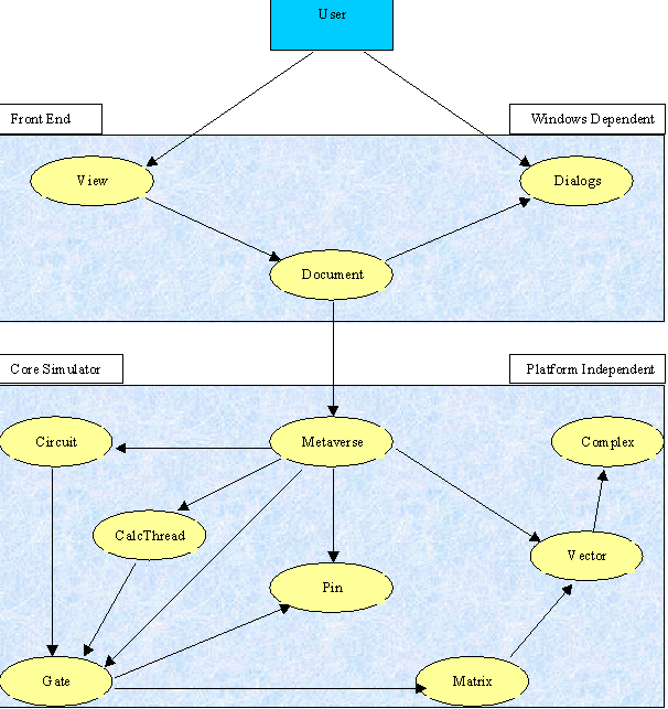
Mfc Derived Classes
|
Class |
Derived From |
Explanation |
|
CQuantumApp |
CWinApp |
Application class. |
|
CQuantumDoc |
CDocument |
Holds the document and performs input and output serialisation. In order to separate the Visual C components from the core simulator a document object in the simulator does not hold the circuit to simulate, as one might expect. Instead it holds a pointer to a circuit and a pointer to a Metaverse which will simulate that circuit. |
|
CQuantumView |
CEditView |
Exposes the view of the document. The user manipulates the view in order to change the document. |
|
CMainFrame |
CFrameWnd |
The main window for the application. Encapsulates the toolbar and status bar. |
Dialog Classes
|
Class |
Explanation |
|
CAboutDlg |
Brings up the credits for the application. |
|
CFactorisationParams |
Asks for parameters for a factorisation such as the number to factorise. |
|
CHaskellEvaluationDialog |
Asks for the parameters to a Haskell simulation, such as Haskell function to evaluate and the input and output format. |
|
CMaxSimpleTestSizeDialog |
Asks the user for the maximum size of the continuous simple tests, which tests are allowed to be run and which simulation algorithms to use. |
|
COptionsDlg |
Asks for program options, such as where to find the Haskell interpreter. |
|
CSimpleTestDialog |
Asks the user which standard simple test circuit is to be loaded and the size of the circuit. |
|
CSimProgress |
Informs the user of the current simulation and the progress to date on that simulation. Optionally shows a graph of the current output state. |
Maths Classes
|
Class |
Derived From |
Explanation |
|
CComplex |
Models a complex number that is stored as real and imaginary components. Also provides mathematical methods to manipulate complex numbers. |
|
|
CBaseComplexVector |
Provides default implementations for mathematical operations on complex vectors. |
|
|
CComplexVector |
CBaseComplexVector |
Models a complex vector with a static array of complex numbers. |
|
CSparseVector |
CBaseComplexVector |
Models a complex vector with a sparse array of complex numbers. |
|
CComplexMatrix |
Models a complex vector, which is an array of complex numbers. Also provides mathematical methods to manipulate complex vectors. |
Gate and Circuit Classes
|
Class |
Derived from |
Explanation |
|
CCircuit |
Models a circuit. A circuit is a list of gates. Each of the gates hold connections between itself and other gates. Provides methods for adding and retrieving gates, loading circuits from input streams, creating standard test circuits and ordering gates. |
|
|
CGate |
Models a gate. A gate holds a list of input and output pins which are exposed to connect to other gates. The CGate class provides only default functionality and it expects derived classes to provides methods for retrieving input and output pins and calculating the output to the gate. |
|
|
CSourceGate |
CGate |
Models a source to the circuit. A source gate is the means by which data enters the system. It has no input pins and only one output pin. CSourceGate provides a default functionality for handling the pins of source gates and expects derived gates to provide the functionality to calculate their outputs. |
|
CStaticSource |
CGate |
A static source is a source gate that has a static output value. It expects a value to be passed to it during construction that tells the gate whether to output a logical 0 or 1. |
|
CRandomisedSource |
CStaticSource |
A randomised source is a source gate which has a random output value set during construction. |
|
CSinkGate |
CGate |
Sink gates are the means by which data leaves the system. They expose one input pin and no output pins. Sink gates do not actually perform any work - they exist only to ensure that pins in all gates in the circuit are connected to another pin. |
|
CInputOutputGate |
CGate |
Input / Output gates are gates which expose a fixed, equal and non-zero number of input and output pins. They encapsulate a matrix that is used to calculate the output for the gate. They provide the functionality to retrieve input and output pins and to calculate the output of the gate given a certain input. |
|
CSquareRootNOT |
CInputOutputGate |
Provides the functionality of the square root of not gate. One input pin and one output pin are exposed. |
|
CFlipGate |
CInputOutputGate |
Provides the functionality of a gate which performs the square root of not on its second input only if its first input is a logical 1. Has two input and two output pins. |
|
CMatrixGate |
CInputOutputGate |
This gate accepts any matrix during its construction. It can have any non-zero and equal number of input and output pins. The gate matrix must be unitary and of the correct size for the number pins that the gate exposes. |
Pin Classes
|
Class |
Derived from |
Explanation |
|
CPin |
Default pin. This is an abstract base class - a derived class must provide the direction of the pin. |
|
|
CInputPin |
CPin |
A pin with an input direction. |
|
COutputPin |
CPin |
A pin with an output direction. |
Simulation Classes
|
Class |
Derived from |
Explanation |
|
SimParams |
Holds the options which are passed to the Metaverse when a simulation is started. There are no methods in this class. |
|
|
CMetaverse |
SimParams |
Provides the methods for performing a simulation. |
|
CCalculationThreads |
Class for creating the threads for the calculation of data. Allows callers to queue calculations to perform. |
|
|
Simdata |
SimParams |
Holds extra options that are passed to Metaverse threads which are going to run a simulation. |
Miscellaneous Classes
|
Class |
Explanation |
|
CQList< class T > |
Provides a template list. Entries in the list are stored in arrays for quick access. It has methods for sorting and searching the list. |
|
CToken |
Used in the parsing of circuit dump files. A token can be a complex number, an integer or a punctuation character. |
|
CGateGroup |
Hold a list of gates. CGateGroup will automatically computer the list of gates whose results they are dependent upon. |
|
CQException |
This provides an exception object that carries a string explaining the cause of the exception. The object can be created from an output string stream that means that any object that has the C++ insertion operator defined can be included in the text. |
User Guide For Quantum
The simulator program, Quantum, is relatively easy to install. It comes with no installation program, though I foresee no difficulties for users in installing and running the application.
There are two versions of the Quantum program. The first version is the release version. The release version is the one that should be used most of the time. It has been compiled with full compiler optimisation and minimal self-tests in order to ensure the maximum execution speed. The debug version has a large amount of self-testing built in. In order to ensure that a program failure reports the maximum amount of information to the user, Automated Tests only work under the debug version of the program.
The Quantum requires the following DLLs to be located in the Windows System directory (Windows 95) or the System32 directory (Windows NT); MFC40.DLL, MSVCRT.DLL, MSVCRT40.DLL. The debug version Quantum requires the following DLLs; MFC40D.DLL, MSVCR40D.DLL. The release DLLs are usually distributed with Windows 95 and Windows NT. All versions of the DLLs are supplied with Microsoft Visual C++ 4.
Quantum is designed to use the features of the Haskell interpreter HUGS. This is widely available from over the Internet. Upon executing Quantum it is necessary to enter the path to the HUGS executable, libraries and a temporary directory for writing files.
The Quantum application itself can be located anywhere.
The screen-shot in Figure 34 below shows the main screen for the Quantum application. The application has a standard Windows interface with a menu and toolbar. The output for a simulation appears in the large window in the centre of the main application window.
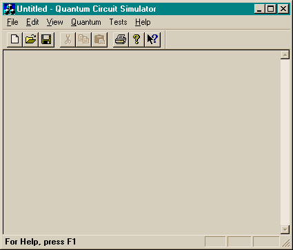
Firstly load the Haskell input file circuit.hs using the Open command on the File menu.
Select the Start Simulation command on the Quantum menu. You will be presented with the dialog box in Figure 35.
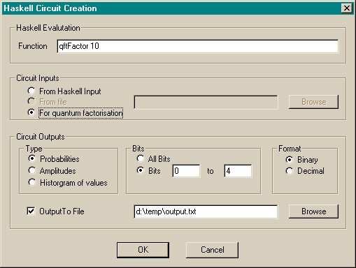
Enter the circuit to evaluate in the Function edit field. If the function is a quantum factorisation function (and it agrees with the implementation described in XXXX) then select the input type ‘For quantum factorisation’. Otherwise leave the selection on ‘From Haskell Input’.
Next, select the type of output format that you require. If you select ‘Probabilities’ the simulation will output the real probabilities of circuit upon completion of the simulation. Selecting Amplitudes results in complex amplitudes being output. Use ‘Histogram of values’ if you want to perform a histogram over the output. This is usually the what you would select if your circuit was made of more than one quantum register and you wanted to output the results of one only register (for instance in quantum factorisation).
Then select the bits that you would like to be output. If you have selected a type of Probabilities or Amplitude then the rest of the output bits are assumed to be zero. For instance, choosing bits 2 to 3 will result in the amplitudes or probabilities of the values 4 to 7 being output. If the type of output is a histogram then you will get a histogram of the probabilities of observing all of the different combinations of the bits that you select. For instance, choosing bits 2 to 3 will output a table containing the probability of observing 00, 01, 10 and 11 on bits 2 and 3.
The Format section allows you to select between outputting values in binary or decimal. ‘Selecting Output To File’ will cause the output of the simulator to be dumped to a file. Leaving this field unselected results in the output being placed in the simulator window.
Select OK to start the simulation. If you have selected the ‘quantum factorisation’ option then you will then be presented with a dialog box (shown in Figure 36) where you can enter the number to factorise. The number to factorise will be constrained by the size of the circuit in accordance with Shor’s algorithm.
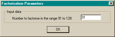
Simulation Progress
During the simulation a progress dialog box will appear. An example is shown in Figure 37. You can terminate the simulation at any time by pressing the Cancel button at the bottom of the box.
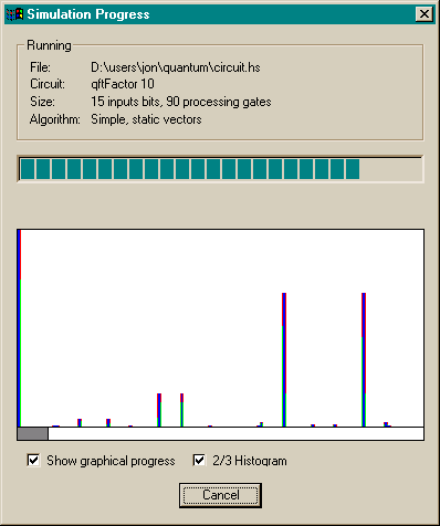
The top section of the dialog box shows information on the simulation being executed and the algorithm being used to simulate the circuit. A progress meter occupies the middle section. At the lower end of the dialog box is a graphical display of the current state of the simulation. The graphical display is turned off by default as can halve the execution speed of the simulation. The ‘Show graphical progress’ check-box allows you to toggle the graphics on or off. The ‘2/3 histogram option’ shows a histogram of the first 2/3 of the circuit and allows a graphical representation of the output from a quantum factorisation. The dialog box can be resized in order to expand the view of the graph.
Each column of pixels in the graphical display is mapped to one or more states in the simulation. Each column is divided in to three areas. The top of the blue area represents the minimum probability obtained across the states that the column represents. The top of the green area represents the average probability of the states and the top of the red area represents the maximum probability.
The example shows a quantum factorisation that is nearly completed. Here you can see the destructive and constructive interference processes at work. Most of the states have no real probability of existing due to destructive interference. The few remaining viable states have been the result of many iterations of constructive interference. The following mural shows the graphs generated by an attempted factorisation.


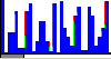
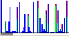
The grey bar at the bottom of the screen shows how many of the probabilities in the state are greater than 0.0001. It shows content of the information in the system and the maximum gains that could be possible using an idealised sparse vector.
Performing a Quantum Factorisation
Load circuit.hs an select the Start Simulation option as described above. In the Function field enter the string "qftFactor n", where n is the size of the first register in the circuit. Suggested values for n range between 6 and 14. Select ‘input for quantum factorisation’. In the output section select the type of histogram and range the histogram over bits 0 to n-1 (i.e. the first register of the machine). Hit OK to proceed and you will be presented another dialog box requesting the number to factorise, as shown in Figure 36.
The simulation will then start and the results will be output to the main window. Notice that the algorithm has only a 50% chance of succeeding on a given iteration.
The option ‘input for quantun factorisation’ performs the mapping whereby the initial state of the system is mapped from |a>|0> to |a>|xa (mod n)>. Ideally the circuit itself would perform this operation. This is left as an exercise for the reader!
Brief descriptions of the commands available on the menu are listed below.
File menu
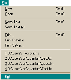
|
Command |
Action |
|
New |
Clears the simulator input files and output text. |
|
Open |
Opens a file describing a circuit |
|
Save Text |
Saves the simulator’s output text |
|
Save Text As |
Saves the simulator’s output text to a specified file |
|
|
Print the simulator’s output text |
|
Print Review |
Review the pages that would be printed |
|
Print Setup |
Set-up the printer |
|
Recent File List |
Allows quick access to the most recently used files. |
|
Exit |
Exit the simulator |
Edit Menu
![]()
|
Command |
Action |
|
Copy |
Copy selected text in to the clipboard |
View Menu

|
Command |
Action |
|
Toolbar |
Toggles the toolbar on or off |
|
Status Bar |
Toggles the status bar on or off |
|
Options |
Brings up the options dialog box |
Quantum
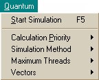
|
Command |
Action |
|
Start Simulation |
Starts simulating the loaded circuit (after presenting the user with options for the simulation) |
|
Calculation Priority |
Sets the priority of calculation thread(s) to either Normal or Below Normal. |
|
Simulation Method |
Sets the simulation method to either Simple or Complex |
|
Maximum Threads |
Sets the number of calculation threads in the complex simulation to a value between one and eight. |
|
Vectors |
Sets the state vector storage method to either static or sparse |
Tests
|
Command |
Action |
|
Single Test Circuit |
Execute a test circuit. The user is prompted with a dialog box asking the type of circuit test. The results are not checked for accuracy. This option is available in both the release and debug versions of the product. |
|
Continuous Circuit Tests |
Execute continuous random circuit tests. The user is prompted with a dialog box asking which tests are to be randomly chosen, their size and the allowed simulation methods. The test results are checked for accuracy. This option is available in the debug version only. |
Help
|
Command |
Action |
|
Help Topics |
Displays the help file. |
|
About quantum |
Displays information on the program. |
The path and file options for the simulation (accessible by the Options command on the View menu) are shown below. You are required to point the simulator at the HUGS executable, libraries and a temporary directory to use while capturing HUGS’s output.
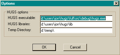
Figure 38
Should the user wish to execute a single test circuit without checking the result for correctness he/she can do so via the Single Circuit Test option on the Test menu. The main use for this option is to provide timings and memory usage information on standard circuits.
Figure 39
Automated Testing (Debug Version Only)
The automated test procedure is described elsewhere in this document. The dialog box below pop up when the Continuous Circuit Tests option is selected on the Tests menu. The user can select which tests are allowed to be run, which algorithms are allowed to be used and the maximum size of the test circuits (in bits). The tests will run continuously until the user intervenes.
Figure 40
module Circuit where
import Complex
import Gates
type Circuit = ( Int, Int, [Gate] )
-- test circuits
notTestCircuit :: Int -> Int -> Circuit
notTestCircuit (n+1) i = (n+1, i, (sqrtGates [0..n]) ++ (sqrtGates [0..n]) )
flipTestCircuit :: Int -> Int -> Circuit
flipTestCircuit (n+1) i = (n+1, i, (flipGates [0..n]) ++ (flipGates [0..n]) )
-- QFT
qft :: Int -> Int -> [Gate]
qft 0 l = [shorRGate 0]
qft n l = (shorRGate n) : (shorSGates (n-1) (l-1)) ++ qft (n-1) l
-- Pure QFT
qftCircuit :: Int -> Int -> Circuit
qftCircuit (n+1) i = (n+1, i, (qft n (n+1)) )
-- Circuit for factorisation
qftFactor :: Int -> Circuit
qftFactor n = ( d, 0, (qft (n-1) n) ++ swapGates [0..n-1] )
where d = n + div (n+1) 2
module Gates where
import Complex
type Gate = ([Int], [Complex Double])
oneOverRootTwo :: Complex Double
oneOverRootTwo = 2**(-0.5) :+ 0
--------------------------------------------------------------------------
-- Matrices
sqrtNotMatrix ::[ Complex Double ]
sqrtNotMatrix = [ oneOverRootTwo, -oneOverRootTwo, oneOverRootTwo, oneOverRootTwo ]
flipMatrix :: [ Complex Double ]
flipMatrix = [ 1, 0, 0, 0
, 0, 1, 0, 0
, 0, 0, oneOverRootTwo, -oneOverRootTwo
, 0, 0, oneOverRootTwo, oneOverRootTwo
]
shorRMatrix :: [ Complex Double ]
shorRMatrix = [ oneOverRootTwo, oneOverRootTwo, oneOverRootTwo, -oneOverRootTwo ]
shorTheta :: Int -> Double
shorTheta n = pi / 2^n
shorSMatrix :: Int -> Int -> [Complex Double]
shorSMatrix j k = [ 1, 0, 0, 0
, 0, 1, 0, 0
, 0, 0, 1, 0
, 0, 0, 0, exp( 0 :+ (shorTheta (k-j)))
]
swapMatrix :: [Complex Double]
swapMatrix = [ 1, 0, 0, 0
, 0, 0, 1, 0
, 0, 1, 0, 0
, 0, 0, 0, 1
]
--------------------------------------------------------------------------
-- sqrtGate n, where n is the bit for the gate to act on
sqrtGate :: Int -> Gate
sqrtGate n = ([n], sqrtNotMatrix)
-- sqrtGates [n]. Constructs a column of sqrtNot gates, where
-- [n] gives the bits to act on
sqrtGates :: [Int] -> [Gate]
sqrtGates [] = []
sqrtGates (b:bs) = (sqrtGate b) : sqrtGates bs
--------------------------------------------------------------------------
flipGate :: (Int, Int) -> Gate
flipGate (a,b) = ([a,b], flipMatrix)
flipGates :: [Int] -> [Gate]
flipGates [] = []
flipGates (b1:b2:bs) = (flipGate (b1,b2)) : flipGates bs
--------------------------------------------------------------------------
-- swaps two bits around
swapGate :: (Int, Int) -> Gate
swapGate (a, b) = ([a, b], swapMatrix)
-- mirrors a circuit around its mid-point
swapGates :: [Int] -> [Gate]
swapGates [] = []
swapGates (b:[]) = []
swapGates (b:bs) = (swapGate (b, last bs)) : swapGates (init bs)
--------------------------------------------------------------------------
-- Gate for the QFT
shorRGate :: Int -> Gate
shorRGate j = ([j], shorRMatrix)
shorSGate :: (Int, Int) -> Gate
shorSGate (j, k) = (([j,k], shorSMatrix j k))
shorSGates :: Int -> Int -> [Gate]
shorSGates j k = if (k>j)
then ((shorSGate (j,k)) : (shorSGates j (k-1)))
else []