Our implementation of RBM uses the single-step contrastive divergence algorithm as discussed, which we will call CD-1, in the “How does it work?” section. There are two phases in CD-1 which we will call the positive and negative phase. This is logically similar to equations (18) and (19) in the “How does it work?” section.

In the positive phase, the input sample “v” from the visible layer is “clamped” to the input layer, and then is propagated to the hidden layer. The result of the hidden layer activation is h.

In the negative phase, “h” from the hidden layer is propagated back to the visible layer with the new v, say v’. This is then propagated back to the hidden layer with activation result “h”.

Using the sampled data, the weights and biases are updated depending on the learning rate which is initialised to 0.5. The learning rate determines, as its name suggests, the rate at which the RBM learns. Increasing the learning rate would mean that the time taken to learn would be much shorted but the data is less accurate. The opposite is the case when the learning rate is low ⁽³⁴⁾. The code for CD-1 can be seen below.

    public void cd_1(double[] input, double learningRate) {
      sampleHidden(input, positiveHMean, positiveHSample);    //positive phase
      gibbsHVH(positiveHMean, negativeVMean, negativeVSample, 
          negativeHMean, negativeHSample); // negative phase
      
      for (int i = 0; i < numHidden; i++) {
        for (int j = 0; j < numVisible; j++) {
                weight[i][j] += learningRate * (positiveHMean[i] * input[j] - negativeHMean[i]
                 * negativeVSample[j]) / numTraining;
        }
      hiddenBias[i] += learningRate * (positiveHSample[i] - negativeHMean[i]) / numTraining;
      }
      for (int i = 0; i < numVisible; i++) {
        visibleBias[i] += learningRate * (input[i] - negativeVSample[i]) / numTraining;
      }
    }
    public void gibbsHVH(double[] hiddenSample, double[] negativeVMean, 
    double[] negativeVSample, double[] negativeHMean, double[] negativeHSample) {
      sampleVisible(hiddenSample, negativeVMean, negativeVSample);
      sampleHidden(negativeVSample, negativeHMean, negativeHSample);
    }
            

In our implementation of the RBM, we perform CD-1 150 times. This is what we will call the “epoch(s)”. It does not refer to the number of Gibbs sampling, which is 1 since it is CD-1, but the number of times the RBM trains over the data. We are utilizing the MNIST data set and that contains 60,000 inputs. The training function with the epoch can be seen below.

    public void train(int trainN) {
      for (int epoch = 0; epoch < trainEpochs; epoch++) {
        for (int i = 0; i < trainN; i++) {
          rbm.cd_1(trainingData[i], learningRate);
        }
      }
    }
    

Once the RBM has been through the training phase, it will then be able to reconstruction from valid input data. For example, if a valid image of 1 is given, the RBM will attempt to replicate it. When reconstructing, the RBM uses its trained weights, biases and the input data to propagate up to create the hidden layer output. Then for each visible layer, RBM propagates down to create the reconstructed image.

    public void reconstruct(double[] visible, double[] reconstructedVisible) {
      for (int i = 0; i < numHidden; i++) {
        hidden[i] = propagateUp(visible, weight[i], hiddenBias[i]);
      }
      for (int i = 0; i < numVisible; i++) {
        double preSigmoidActivation = 0.0;
        for (int j = 0; j < numHidden; j++) {
            preSigmoidActivation += weight[j][i] * hidden[j];
        }
        preSigmoidActivation += visibleBias[i];
        reconstructedVisible[i] = sigmoid(preSigmoidActivation);
      }
    }
       

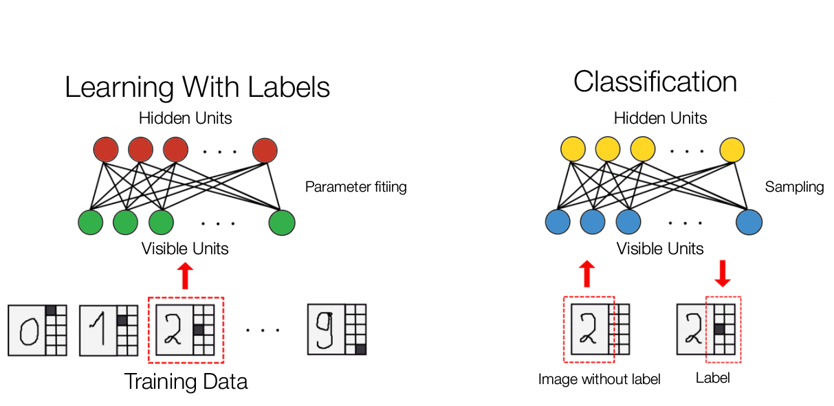
Classification depends on reconstruction. We can feed the RBM the images without labels and when the given input is reconstructed, there will be values generated at the label ⁽⁹⁾. The largest unit in the label is the value RBM classifies the given image as. The image below describes this process:

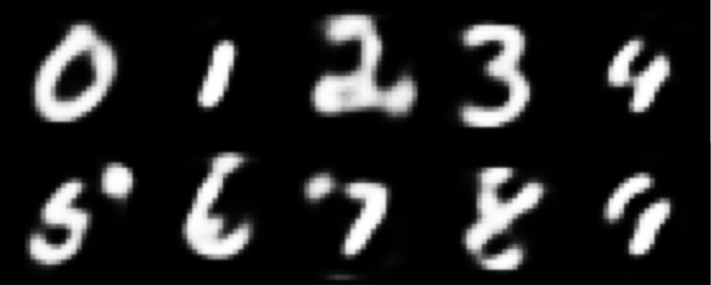
As the RBM is a generative model, it should be, in theory, possible to look “into the mind of a neural network”⁽⁸⁾. We decided to implement a somewhat simpler version to generate from our RBM the digits.

First we tried “clamping” ⁽⁸⁾ the corresponding label unit to 1.0 and all of the other visible units to 0.0. Using the reconstruction as explained above, we generated the image. However, there was an issue with the reconstructed image being unclear, as the RBM was only turning on 1 / 794 of the visible nodes. This meant that the hidden units struggled to activate and thus reconstructed a poor image.

In order to overcome this issue, we amplified the input data to 794.0, to compensate for the lack of visible nodes turned on. We then “clamped” the corresponding label unit again in the reconstructed data by setting the corresponding label to 1.0 and the other label units to 0.0. We reconstruct this again and again until the image is clear (In this case, it was regenerated 5 times).

This is the result of the regeneration from the label data.