On the Internals of Stream Processing Systems
Architecture, Threading Model and Performance
 Image credit: Unsplash
Table of Contents
Stream Processing Systems (SPSs) are an integral part of modern data-intensive companies. In a world where streams are becoming king, they are commonly employed for much more than data analytics. An example is DriveTribe, a social network whos entire backend is implemented as a stream processing job, but they are also used for many other event-driven applications.
When I began working on Clonos, a novel local recovery and high-availability approach for SPSs, I knew very little about the internals of SPSs. But now, I needed to modify one quite heavily and that would require a good mental model of their design. I understood what SPSs did from a theoretical standpoint and I had even used them extensively in previous projects, but I had no clue about their internal design. I scoured the internet for resources, and while I was able to piece together a little bit of what was going on, in the end I would need to spend weeks looking through the code of an SPS before feeling confident enough to start designing Clonos.
While Database Management Systems (DBMSs) architecure has been extensively studied and discussed in papers and books, the architecture of SPSs has not. I believe the reasons for this are that SPSs are actually fairly simple once a few mental hurdles are overcome and that not a lot of variation exists between different SPSs. For this reason, while this post is based on my experience with Apache Flink 1.7, it will hopefully be useful to researchers working on any SPS.
For this post, I assume only familiarity with SPSs from a user perspective.
Stream Processing Systems
We will begin by discussing a few background concepts on Dataflow systems needed to understand the remainder of this post. These may be skipped if familiar. Then, we will discuss the distributed components of an SPS and finally we will move on to the local runtime which executes each task.
Dataflow Graphs
SPSs are often dataflow systems in that they execute dataflow programs. Dataflow programs are structured as flows of data between a Directed Acyclic Graph (DAG) of operators.
Each of these operators applies a transformation to a stream of data records, which are composed of:
- Content: A (generally) flat datastructure of arbitrary data which the program processes.
- Key: A form of identifier (think userID/itemID/userRegion) assigning the record to a logical “group”. Used for routing and aggregating.
- Timestamp: The timestamp at which the record either entered the system, is being processed or was created. The different semantics are a discussion for another day. Used for time-based operations in windows.
Structuring programs this way allows for easier scaling through the use of both data parallelism and pipeline parallelism.
These dataflow programs are defined using either imperative (Flink’s DataStream API) or declarative (SQL) APIs. For this section, consider the simple example of a streaming word-count shown below.
//pseudo-code for defining a Flink Dataflow program using the Streaming (DataStream) API
//Example is WordCount with initial filtering.
env.source(new MySource(...))
	.filter(x => x.last == ".") //filter out only well-punctuated sentences
	.flatMap(new MyTokenizer()) //split sentences into tokens
	.keyBy(0) //Group records by token (words)
	.sum(1) //Reduce using the second property of the record (count)
	.sink(new MySink(...))
When submitted, the SPS translates this program into a high-level plan called a logical dataflow, which contains the DAG of operators, but lacks information such as the actual algorithmic implementation of each operator. The logical dataflow generated from the example code is shown below in Figure 1.
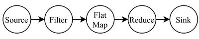
You can see how by having a single processing unit execute each logical operator, one would already exploit pipeline parallelism, increasing throughput. However, sometimes a few operators require more horsepower in order for the pipeline to run smoothly. This can happen for a few reasons:
- The upstream operator is faster than the downstream operator.
- The downstream operator has to process more records than the upstream operator (e.g.: the upstream is a FlatMap operator)
- The downstream operator requires more memory.
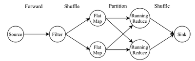
For these and other reasons, the system may choose to increase the parallelism of a few operators. The user can also often provide hints of desired parallelism. This and other runtime information is combined in order to generate the physical plan or physical dataflow which the system will execute. This includes the algorithmic implementations of operators, parallelism of each operator and even information on how data should be shared from one logical operator to the next (see Figure 2). Network connection types include:
- Forward: Each physical operator instance i forwards to the following operators i’th instance. Generally only possible when two adjacent operators share the same parallelism.
- Shuffle: Randomly (or effectively randomly) send data to one downstream physical instance. Useful for rebalancing load after a change in parallelism.
- Partition: Use the record key to send the record to the downstream physical operator instance handeling that key.
One step we skipped here is optimization. SPSs will often transparently optimize the dataflow programs for better throughput or latency. A simple example of this is pushing “selective” (e.g.: filter) operators as far upstream as possible without changing the semantics of the program. This helps reduce the data-volume of the entire program.
Finally, remember that operators are mostly just mathematical descriptions of what can happen in such an operator. For example, the MapOperator simply knows that it receives one input record and outputs one output record in response. What happens is provided by a user-defined function (UDF) which the operator owns.
Tasks & Thread Model
When the physical plan is submitted for execution, pipelines of operators connected by forward connections are identified by the system and grouped into an OperatorChain. Operator chains are thus broken by pipeline breakers such as a change in parallelism, partition or shuffle network connection.
When a record is fed to an OperatorChain, that record flows through all operators until it exits the chain. The way this works internally is that the OutputCollector of each operator immediately calls the following operator.
Each operator chain will be hosted by a Task, which will be responsible for all aspects of that chain (scheduling, state management, fault-tolerance and networking).
OperatorChain to have length 1.
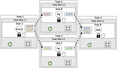
As shown in Figure 3, each TaskSlot provides a task with a single execution thread (the green arrow) and a memory segment (the squares in a square) for the tasks operations.
This way, one can perform capacity planning quite easily by defining the memory that each TaskSlot should provide.
The thread model of SPSs is thus that simple: split the workload (either randomly or by key) into Tasks and let each Task execute on a single thread with no need for synchronization which would slow it down.
Of course, there are a few more threads in the system used for networking and checkpointing, which we will discuss below. And as shown in Figure 3, there is at least one lock for each Task, but as you will see, there is very little contention on it.
Distributed Components
With the terminology defined, let’s take a detour and discuss the high-level distributed runtime of an SPS, before coming back to how execution is driven for each task.
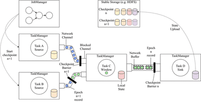
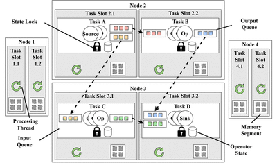
The image above shows a simplified version of Flink’s distributed runtime components, of which there are three:
- TaskManagers: Host dataflow tasks in their
TaskSlots and execute the computation itself. - JobManager: Oversees the execution of the job, scheduling the
Tasks to availableTaskSlots, triggering checkpoints and handling failures. - Stable Storage: An external component used to store checkpoints. In this case, we use HDFS.
Not depicted in the image are the data source and sink (not to be confused with the source and sink operators) of the dataflow. Commonly, streaming storage solutions such as Kafka are used for this.
The example dataflow graph for this section is constituted by two tasks containing source operators, one task containing a window operator and one task containing a sink operator. The network channels between TaskManagers are also shown containing streams of records flowing between them.
For increased performance records are often serialized into NetworkBuffers, and it is those buffers that are sent across the network between TaskManagers.
By sending large buffers instead of small records, we reduce the number of system calls performed, improving performance.
Periodically, the JobManager will perform an RPC on the TaskManagers which host the source operators, announcing that they should begin a checkpoint. This will cause these Tasks to checkpoint their state and upload it to HDFS. We will explore this more in depth later.
Scheduling
The prior example assumes for simplicity that each TaskManager has only one TaskSlot, however this is not commonly the case.
Scheduling then becomes a concern as one could change properties of the execution of the dataflow by changing how Tasks are assigned.
Let us now instead assume the existance of 4 TaskManagers, each with 2 TaskSlots (a total of 8 slots available) upon which we have to schedule 4 Tasks.
If one wanted to maximize the availability of the dataflow, one would place one Task on each TaskManager, as shown below in Figure 5. This is also true if we wanted to maximize load balance.
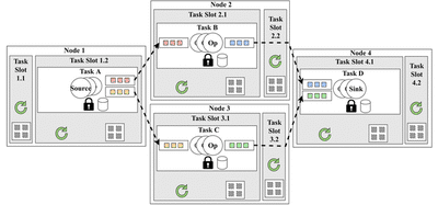
On the other hand, if we wanted to instead maximize performance, we would likely place the connected Tasks with the greatest data-volume in the same TaskManager, thus reducing the amount of data which needs to be sent accross the network. This way, only a pointer to the data buffer must be passed around.
TaskManager Runtime
We can finally get into the meat of this post, the TaskManager runtime, and see how execution is driven for a single Task, this is shown below in Figure 7.
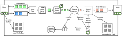
This Figure zooms into the Window task in Figure 4. Since it has 2 upstream tasks, there are two input queues where data buffers are placed.
Netty is what Flink uses for its dataplane networking. Netty reads buffers from the network and places them in these queues. Though the Netty runtime has a large thread pool, each logical network channel can only be owned by a single thread at a time, thus removing the need for locking.
The buffers are obtained from the Input Buffer Pool which is created from the TaskSlot’s buffer pool. The same is true for the Output Buffer Pool.
The buffers sit in this queue until they are needed. Driving the execution of the Task is the StreamInputProcessor (represented with a thread arrow). This is the class which actually contains an infinite while-loop for processing input data buffers. Whenever a new buffer is needed, it is requested from the CheckpointBarrierHandler, which requests it from the InputGate. The InputGate then chooses one of the queues from which to take a buffer.
When the buffer reaches the StreamInputProcessor again, it is passed to the deserializers, which then spit out the records one by one, which are fed to the Operator itself until the buffer is exhausted.
Before we move on to what happens when records are processed, let me explain some components we skipped over. The InputGate is simply an abstraction which unites all input channels, providing a getNextBuffer() functionality. The CheckpointBarrierHandler wraps the InputGate and blocks the flow of buffers whenever a checkpoint barrier is found on that channel.
Whenever the CheckpointBarrierHandler identifies that all channels are blocked by a barrier, a local state snapshot is created and uploaded to HDFS. In most modern SPSs, this is done in an asynchronous way:
- The state lock is acquired (there should be no contention on it generally).
- A copy of the state is created: either through an in-memory copy or using the capabilities of the backing datastore (MVCC datastores).
- The state lock is released.
- A thread is created to upload the state copy.
- Concurrently to 4, normal processing continues.
The state lock must be acquired by any thread which wants to access the operator state. Generally, this is only the StreamInputProcessor thread which drives the Task, and as such there is no contention. However, RPCs can be received which access the state such as begin checkpoint RPCs or state query RPCs. More commonly, the TimerService may asynchronously trigger a Timer, which will race the main thread for access to the state.
Circling back to the Operator, as it receives records, it passes them to the UDF which it contains, and the generated outputs are passed to the RecordWriter, which serializes the records into output buffers.
As you can see in more detail, the thread model is still very simple: A single processing thread, a few network (dataplane and controlplane) threads and a few timer threads interact in simple ways. A single lock guarantees consistent access to the Task state.
Other Performance Considerations
In this Section, I will leave a few notes on performance aspects which I find relevant.
Network
Netty is a mature and complex project by itself, however it is deeply intertwined with Flink and its performance. While I am no Netty expert, here are a few Netty aspects which were extremely useful whilst developing the ThreadCausalLog datastructure:
- Allows for out-of-heap buffers. Avoids copying data from JVM heap memory to OS memory.
- Highly optimized and useful byte buffer datastructures (
ByteBuf) help reduce data copies.- Slices allow for views over existing buffers, without copying.
- CompositeByteBufs allow one to make complex buffers composed of other buffers, again without copies.
- The use of Buffer Pools and reference counting helps avoid allocation overhead.
- The event-driven architecture ensures no wasted computation.
State
Flink and other SPSs often allow for pluggable StateBackends. This means they can make use of the most performant datastores, even when working with larger-than-memory state.
This is relevant because disks are extremely slow. Flink users typically use the RocksDB StateBackend, though more streaming focused backends are emerging, such as FASTER.
These StateBackends use LSM Tree as their primary datastructure, which makes them attractive for write-heavy workloads such as streaming state updates (as opposed to the more common B+ tree).
Execution
The Flink codebase contains occasional warnings regarding function inlining, a technique which aims to reduce the number of function calls performed. Each function call adds a bit of overhead from managing stackframes and jumping around in the code segment. Though I am not sure how it works, it seems one can hint at the JVM that one wants a piece of code to be inlined by making it fairly small.
End Notes
There is, of course, so much more to say about the design of SPSs.
We only scratched the surface of state management in SPSs. See (Citation: Carbone & al., 2017) Carbone, P., Ewen, S., Fóra, G., Haridi, S., Richter, S. & Tzoumas, K. (2017). State management in Apache Flink®: consistent stateful distributed stream processing. Proceedings of the VLDB Endowment, 10(12). 1718–1729. for an overview of state management in Flink. For the asynchronous checkpointing algorithm that Flink uses see (Citation: Carbone & al., 2015) Carbone, P., Fóra, G., Ewen, S., Haridi, S. & Tzoumas, K. (2015). Lightweight asynchronous snapshots for distributed dataflows. arXiv preprint arXiv:1506.08603. .
One of the big use-cases in SPSs is windowing and as such large performance gains can be obtained simply through better windowing algorithms (Citation: Traub & al., 2021) Traub, J., Grulich, P., Cuéllar, A., Breß, S., Katsifodimos, A., Rabl, T. & Markl, V. (2021). Scotty: General and Efficient Open-source Window Aggregation for Stream Processing Systems. ACM Transactions on Database Systems, 46(1). 1–46. https://doi.org/10.1145/3433675 .
If you would like a deeper look at the theory behind SPS fault-tolerance, I would recommend reading through my MSc Thesis up to Chapter 3.2.1.1 (skipping Chapters on fault-tolerance), as it starts from basically zero (the Message Passing System model).
One aspect of performance we did not mention is hardware acceleration. See Saber (Citation: Koliousis & al., 2016) Koliousis, A., Weidlich, M., Castro Fernandez, R., Wolf, A., Costa, P. & Pietzuch, P. (2016). Saber: Window-based hybrid stream processing for heterogeneous architectures. for an example of a highly performant scale-up (yes, scale-up) SPS using HW acceleration. Even in 2021, this is still an open research direction.
One final note is optimization, which we barely touched. I don’t know a good resource to direct you to, but optimization can lead to enormous performance gains for free.
Cited Bibliography
- Carbone, Fóra, Ewen, Haridi & Tzoumas (2015)
- Carbone, P., Fóra, G., Ewen, S., Haridi, S. & Tzoumas, K. (2015). Lightweight asynchronous snapshots for distributed dataflows. arXiv preprint arXiv:1506.08603.
- Koliousis, Weidlich, Castro Fernandez, Wolf, Costa & Pietzuch (2016)
- Koliousis, A., Weidlich, M., Castro Fernandez, R., Wolf, A., Costa, P. & Pietzuch, P. (2016). Saber: Window-based hybrid stream processing for heterogeneous architectures.
- Traub, Grulich, Cuéllar, Breß, Katsifodimos, Rabl & Markl (2021)
- Traub, J., Grulich, P., Cuéllar, A., Breß, S., Katsifodimos, A., Rabl, T. & Markl, V. (2021). Scotty: General and Efficient Open-source Window Aggregation for Stream Processing Systems. ACM Transactions on Database Systems, 46(1). 1–46. https://doi.org/10.1145/3433675
- Carbone, Ewen, Fóra, Haridi, Richter & Tzoumas (2017)
- Carbone, P., Ewen, S., Fóra, G., Haridi, S., Richter, S. & Tzoumas, K. (2017). State management in Apache Flink®: consistent stateful distributed stream processing. Proceedings of the VLDB Endowment, 10(12). 1718–1729.
Pedro F. Silvestre
PhD Student at Imperial College London
My research interests include all kinds of performant and distributed data-intensive systems.