A sparse matrix is one with a large proportion of zero elements. Many
important algorithms involve multiplying a sparse matrix by a vector, ![]() .
This key computational ``kernel'' is the focus of the main laboratory
project for this course.
.
This key computational ``kernel'' is the focus of the main laboratory
project for this course.
Applications include:
   double A[A_rows][A_cols];
   double x[A_rows], y[A_rows];

   for ( i=0; i<A_rows; i++ ) {
      sum = 0.0;
      for ( k=1; k<=A_cols; k++ )
        sum += A[i][k]*x[k];
      y[i] = sum;
   }
To make this sparse we need to choose a storage scheme. A popular choice is ``compressed row'':
    struct MatrixElement {
      long col;
      double val;
    };
    /* no of non-zeroes in each row */
    int SA_entries[A_rows];

    /* array of pointers to list of non-zeroes in each row */
    MatrixElement** SA = (struct MatrixElement**)malloc(sizeof(struct MatrixElement)*A_rows);

    /* When SA_entries is known we can allocate just enough memory for data */
    for(i=0; i<A_rows; i++) {
      SA[i] = (struct MatrixElement*)malloc(sizeof(struct MatrixElement)*A_entries[i]);
    }
The idea here is that for each row, we keep an array of the non-zero
matrix elements, pointed to by SA[i]. For each element
SA[i][j] we need its value, and its column number. So, if
A[i][j] is the nth non-zero in row i, its value
will be stored at SA[i][n].val, and SA[i][n].col will be
j.
Now the matrix-vector multiply can be written as:
    for(i=0; i<A_rows; i++) {
      sum = 0;
      for(j=0; j<SA_entries[i]; j++) {
        sum += ((SA[i][j]).val)*x[(SA[i][j]).col];
      }
      y[i] = sum;
    }
You can find the source code in
/homes/phjk/ToyPrograms/C/smv-V1Copy this directory tree to your own directory:
cd
cp -r /homes/phjk/ToyPrograms/C/smv-V1 ./
Now run some setup scripts:
cd smv-V1
source SOURCEME.csh
./scripts/PutInputFilesOnLocalDisk.sh
./scripts/MakeMatrices.sh 1 2 3
This creates a directory /tmp/USERNAME/spmv/ and builds some sample matrices there. You should compile the application using the following commands:
cd solver/csteady/
make
Now you can run the program:
./csteady ../../inputs/courier1/ ../../inputs/courier1/STEADYThis reads input from the directory for problem size 1, and writes its output to a file called ``STEADY'' in the same directory. This is problem size 1 - very tiny. Problem size 3 is more substantial. 1
Try to make sure no other processes are active as they will interfere with your results. How many times do you need to repeat your experiments to get a reliable result?
cachegrind ./solver/csteady/csteady inputs/courier1/ inputs/courier1/STEADY
cachegrind --L2=64,1,16 ./solver/csteady/csteady inputs/courier1/ inputs/courier1/STEADY}This simulates a 1-way (ie direct-mapped) cache with 64, 16 byte lines. Now replace 64 with powers of two up to
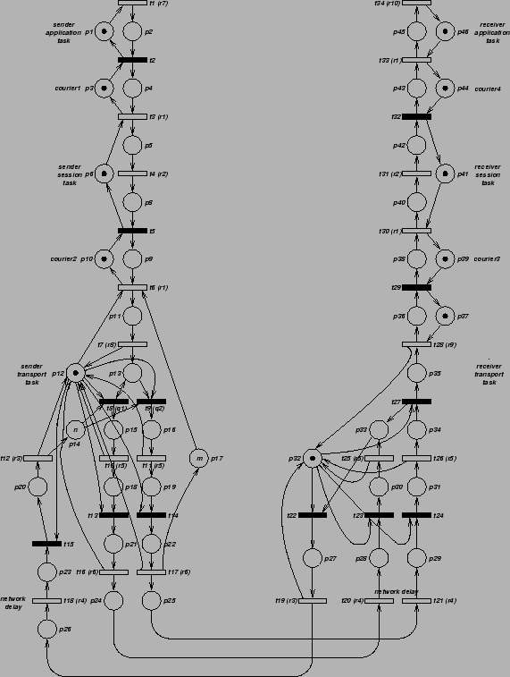 |
The program solves a Markov chain derived from a probabilistic Petri model (see see Figure 1) of a simple communication protocol. The problem size corresponds to the protocol's ``window size'' - the number of messages which can be in sent before the transmitter blocks awaiting acknowledgement. Execute the following commands to see the final results:
cd inputs/courier1
./perf
The output shows the values for the following metrics of the protocol's performance:
Run cachegrind over a range of parameters you need to write a shell script. You might find the following Bash script useful:
#!/bin/bash -f

for ((x=64; x <= 1048576 ; x *= 2))
do
  echo -n ``Size $x ``
  cachegrind --D1=$x,1,16 ./solver/csteady/csteady inputs/courier1/ inputs/courier1/STEADY \
  2>&1 | grep ``D1  miss rate''
done
(The final line combines stdout and stderr and selects just the D1 miss rate from the simulation output). You can run this script by typing
./scripts/cg-loop.sh > resultsThis writes all the results to a file ``results''. It takes quite a while!
You need to convert the ``results'' file to a neat table of problem size against performance. Try:
awk '{print $2, $6, $8, $10}' <results > table
This picks out the miss rate data columns. The output
is sent to the file ``table''.
Try using the gnuplot program. Type ``gnuplot''. Then, at its prompt type:
plot 'table' with linespoints
plot 'table' using 0:2 with linespoints, 'table' using 0:3 w lp, 'table' u 0:4 w lp
Paul Kelly, Imperial College London, 2004