ARGraphs Cell Nucleus Segmentation Codes

ARGraphs Cell Nucleus Segmentation

Relevant Paper: S. Arslan, T. Ersahin, R. Cetin-Atalay, and C. Gunduz-Demir, "Attributed relational graphs for cell nucleus segmentation in fluorescence microscopy images," IEEE Transactions on Medical Imaging, vol. 32, no. 6, pp. 1121-1131, 2013. [source] [pdf] [bibtex]

C implementation of the cell nucleus segmentation algorithm using attributed relation graphs. The program has two modes: cell nucleus localization (marker primitive definition) and region growing (flooding) for boundary delineation. First, it should be run in cell nucleus localization mode to roughly find cell nuclei and four types of primitives, which are then used in the second stage for segmentation of nuclei. The usage of the program and the parameters are briefly explained here. Please note that, all the parameters should be entered properly, since no default values were defined. We tested the program on Ubuntu and Mac OS X machines, but it should be also applicable to Windows platforms. The following tutorial is for Unix-based (Linux, Mac) terminals.

Download Codes Github

Compiling C Codes

Before using ARGraphs segmentation codes, you should compile the c and h files. We recommend that you use the standard gcc compiler for compilation shown as below:

$ gcc *.c src/*.c -o ARGraphs –w

(IMPORTANT: Linux/Unix users, if you get any errors, please replace -w with -lm)

First Run: Cell Nucleus Localization Mode

After obtaining your binary named as ARGraphs you may call the program from the command line as follows:

$ ./ARGraphs <0> <1> <2> <3> <4> <5> <6> <7> <8>

Parameters:

<0> The flag for switching between two modes. For cell nucleus localization mode, it should be set to 1 and for cell nucleus segmentation (flooding) mode, it should be set to 2. Please note that, it is not possible to run cell nucleus segmentation (flooding) mode before obtaining the primitives. The following parameters are valid if this parameter’s value is set to 1.
<1> The name of the 2D gray image which will be processed. The first row of the file should contain the dimensions of the image separated by a whitespace. For example, for an image with 768x1024 resolution, the first row of the file should be 768 1024.
<2> The name of the initial segmentation mask, which is used to determine local Sobel thresholds for primitive definition. Please note that, any mask should be used here, as far as it covers the cellular regions. The mask should have the same dimensions as the 2D gray image. Similarly, the first row of the file should contain the dimensions of the mask, separated by a whitespace. If you would like to use our initial segmentation map, you can find the Matlab® function in the matlab folder or here.
<3> The name of the output file which will contain the localized cell nuclei (primitive markers). The program will save the file in the same format as the input files, where the first row will contain the dimensions of the image separated by a whitespace. All objects in the file are labeled with unique ids.
<4> T_size, primitive length threshold parameter used in the primitive definition and graph construction stages. Note that for fluorescence microscopy images taken with a 20x microscope objective lens and 768x1024 image resolution, we set this value to 15, considering the sizes of cell nuclei in the image. You should change this value according to your images.
<5> T_perc, percentage threshold used in the iterative search. Smaller values of this parameter yield more false detections.
<6> T_std, standard deviation threshold used in nucleus localization. When smaller thresholds are used, the nucleus candidates need to be rounder to be detected.
<7> The number of the connected component to be processed. The program runs independently for each connected component of the mask. This parameter should be set to -1 for processing the whole image.
<8> Option for creating extra output. Setting it to 0 will only produce localized cell nuclei (primitive markers) which roughly represent cell nuclei. For flooding, the program needs the final primitives; therefore it should be set to 2. For getting only initial primitives, it should be set to 1.

For example the following call will produce localized cells and primitives for guiding the region growing process in the second stage (assuming the name of the binary file is ARGraphs).

$ ./ARGraphs 1 blue mask prim 15 0.3 4 -1 2

Second Run: Region Growing (Flooding) for Cell Boundary Delineation

You may call the program from the command line as follows:

$ ./ARGraphs <0> <1> <2> <3> <4> <5>

Parameters:

For example the following call will produce the boundaries of segmented cell nuclei.

$ ./ARGraphs 2 prim mask 5 segmented_cells 0

How to Visualize the Segmented Boundaries

All the files produced by this program contain the number of dimensions in their first rows. They can be easily read using Matlab®. For example, an output file which contains segmented cell nuclei, named segmented_cells, is read and demonstrated as follows:

>> seg = dlmread('segmented_cells', '', 1, 0);
>> figure, imshow(label2rgb(seg, 'jet'));

Example Run on Provided Sample Images

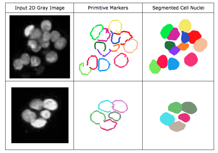
You can run the program with the provided files (blue4, mask4) in the data folder using the following parameters. T_length: 15, T_perc = 0.3, T_std = 4, and W = 5.

The results would look like similar to those of example subimages. Note that the sizes of the images from which they are cropped are the same and that we run the algorithm on the original-sized images. The original images were taken with a 20x microscope objective lens and 768x1024 image resolution.

$ gcc *.c ../*.c -o ARGraphs –w
$ ./ARGraphs 1 ../data/blue4 ../data/mask4 out_prim 15 0.3 4 -1 2
$ ./ARGraphs 2 out_prim ../data/mask4 5 ../data/segmented_cells 0