Building Spiking Neural Networks
In this post, I will go over the code available in this repository that implements Izhikevich neurons as its neuron model. But before we dive into the code let’s try to appreciate what we are trying to actually simulate: biological neurons. It’s important to understand the real world before we get all tech savvy and put on our hacker attitude on.
Source: Wikimedia Commons
These neurons are what we find in the living realm, yes there is a natural world out there beyond social media and the computer screen. Your brain is built from billions of these neurons, billions! Although there are variants of them structure and behaviour wise, they all essentially work in the following steps:
- The neuron maintains a resting potential often around -65 millivolts on its membrane when left alone. That is the voltage difference between inside of the cell (purple area in the diagram) and outside of it. This is created by ion channels on the membrane that allow certain ions such as sodium and potassium to pass or not pass through.
- When this membrane potential reaches a critical threshold, it causes the ion channels to open and create a sudden and sharp rise in the voltage difference. In neuroscience it is the action potential, for simplicity we will refer to the phenomenon as the neuron firing or emitting a spike.
- This sharp potential increase, a.k.a. spike, cascades down the axon of the neuron travelling to the axon terminal where it connects to other neurons’ dendrites. What happens when an action potential reaches the axon terminal? Good question.
- When the action potential reaches the axon terminal, the voltage triggered channels open and neurotransmitters are released into the synapse. These neurotransmitters then bind to the receivers on the dendrites on the connected neurons. These channels are often what gets messed up, kept open or closed beyond normal levels,when people take drugs like caffeine.
- The incoming neurotransmitters cause the membrane potential to increase. Once the it reaches a threshold, as in enough previous neurons fire, a new action potential is created.
- The spiking neural network attempts to capture these cascading spikes and we computationally try to model the membrane potential to simulate a biological network.
Source: Wikimedia Commons
The main point behind a computation model of a biological neuron is the behaviour of the membrane potential. Since we don’t have infinite resources, at least I don’t, we need to compromise between how closely we want to follow the biological setting and efficiently compute it. There are many biological neuron models that trade realism and efficiency. On the most efficient side, we have integrate-and-fire models which simply accumulate, integrate, the incoming current from previous neurons and check if it passes a threshold to fire. On the other end of the spectrum we have Hodgkin–Huxley model that meticulously computes the ionic flows (potassium, sodium, etc.) to compute the membrane potential. The authors Hodgkin and Huxley were awarded the 1963 Nobel Prize in Physiology or Medicine for their work.
Summing up incoming current is too simple and not biologically realistic, whereas Hodgkin-Huxley is very realistic but expensive to compute all those ionic flows. This is why Eugene Izhikevich came up with his model in the paper titled Simple Model of Spiking Neurons. It was designed to strike a balance between computational efficiency and biological realism. This is the model we will use to build our spiking neural network. Let’s have a look at what the fuss is all about:
$$ \begin{aligned} \frac{dv}{dt} &= 0.0v^2 + 5v + 140 - u + I \\ \frac{du}{dt} &= a(bv-u) \\ \end{aligned} $$which describes how the membrane potential $v$ changes over time (hence it is a differential equation). The $I$ is the input current to the neuron which could be an accumulation of incoming spikes. Where do these magic numbers come from? Izhikevich fits them to match an actual biological neuron to get the voltage to be in millivolts and the time to have units milliseconds. For the details on what these parameters represent and how they change the behaviour of the neuron you can refer to the paper. The main types we are interested are excitatory and inhibitory neurons. As their name suggest, the former increases the membrane voltage of the neurons it connects to while the latter decreases it. The parameters $a,b,c,d$ try to capture the different dynamics of neurons we observe in nature.
When the value of $v$ reaches a threshold, in this case it is set to $v \ge 30$, the following happens:
$$ \begin{aligned} v &= c \\ u &= u + d \end{aligned} $$which in essence resets the neuron so it can fire again depending on the incoming current. Now all we have to do is iteratively compute this membrane potential and see which neurons fire in a network of them. To complete the network we need a few more things, specifically:
- A number of excitatory and inhibitory neurons, we’ll refer to this as $x=1$ if excitatory, $x=0$ inhibitory.
- Their $a,b,c,d$ parameters so we can compute their behaviour.
- The weights / connections between these neurons, the topology of the network.
- The delays of the connections, i.e. the time it takes for the spike to reach a connecting neuron.
However, we can perform an optimisation and compress the $a,b,c,d$ into a single $0 \le r \le 1$ parameter:
$$ \begin{aligned} a &= 0.02x + (1-x)(0.02+0.08r) \\ b &= 0.2x + (1-x)(0.25-0.5r) \\ c &= x(-65+15r^2) + -65(1-x) \\ d &= x(8-6r^2) + 2(1-x) \end{aligned} $$which capture enough variation in the behaviour of the neurons that we want to model. For more details you can refer to the paper. Great, all is set. Now we need to figure out how to compute the membrane potential $v$ over time. Recall that the equation we are given is a differential equation that describes how it evolves over time. So given some initial state, we want to compute, approximate its value over time. Since our computers run in discrete steps, we can just chuck these equations in a calculator and expect it to spit out some smooth calculation of the membrane potential over time. What should catch your attention is the word smooth. When we try to simulate mother nature which runs in real time, in a computer that computes things step by step, we will get an approximation and how close / smooth that is depends on the resolution we have. In other words, it depends on how small our discrete computation steps are.
This brings us to Euler’s Method, a numerical method to solve the differential equation we have for the membrane potential $v$. Recall our objective: we want to compute the value of $v$ over time and record whenever it passes the threshold. The membrane potential is a function of time $f(t) = v$ and we are given its derivative $f'(t) = \frac{dv}{dt}$ which describes how it changes over time. For the moment we are ignoring $u$ since we will apply the same method.
Here is the crux of the matter. If $f'(t)$ tells us how much the function changes at that point in time, then why don’t we make a small step $h$ using it to update $f(t)$ and repeat.
Sure, there is a mathematical derivation to justify how this approximates the integral but we’ll leave that as further reading. The situation we have for spiking neural networks and computing this membrane potential business is:
$$ f(t+h) \approx f(t) + hf'(t) $$which says the value is updated by how much we think is going to change now $f'(t)$ with how big of a step we want to take $h$. Let’s take a concrete example before we apply this to the actual neuron model equations. Let’s assume for now $f(t) = e^t$ and thus $f'(t) = e^t$. If you are like me and forget derivatives and things, the derivative of $e^x$ is $e^x$ so we get those equations. Now we want to know the value of $f(2)$ starting with $f(0) = 1$. Why is it one? No tricks here: $e^0 = 1$. We just evaluated the initial value. Picking $h=0.5$, we get:
| t | e^t | f(t) | f’(t) | hf’(t) | f(t+h) |
|---|---|---|---|---|---|
| 0.0 | 1.00 | 1.0 | 1.00 | 0.5 | 1.5 |
| 0.5 | 1.65 | 1.5 | 1.65 | 0.825 | 2.325 |
| 1.0 | 2.72 | 2.325 | 2.72 | 1.36 | 3.685 |
| 1.5 | 4.48 | 3.685 | 4.48 | 2.24 | 5.925 |
| 2.0 | 7.39 | 5.925 | 7.39 | 3.695 | 9.62 |
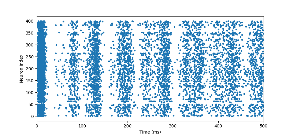
so we approximate our actual function $e^t$ with finite number of steps $f(t)$. You’ll notice that we under approximated it because we took coarse steps $h=0.5$. If we decrease $h$, our approximation will get close to the actual value albeit at more computation cost. With the Euler’s Method we have everything we need to now simulate and obtain spike trains shown below:
spiketrain
where we observe at which time point which neuron fired. In this case, we see an oscillatory behaviour which is very common in brains. Below is the original code with extra annotations that computed that simulation:
def izhinet(params: dict, in_current: np.ndarray, runtime: int, deltat: float) -> np.ndarray:
  """Simulate Izhikevich Networks with given parameters."""
  # params['ntypes'] (N,) True for excitatory, False for inhibitory, the x from the equations
  # params['nrands'] (N,) the r
  # params['weights'] (N, N) connecting weights
  # params['delays'] (N, N) connection delays
  # in_current (B, N) input current, where B is batch size so we can simulate the same network
  # with different inputs.
  ntypes = params['ntypes'] # (N,)
  nrands = params['nrands'] # (N,)
  # We will look back in time, so need to transpose these. The original parameters tell us
  # for example the delay from ith neuron to jth neuron. We need the delay back in time so
  # we can compute how further back we need to look for jth neuron to receive from the ith neuron
  recv_weights = params['weights'].T # (N, N)
  recv_delays = params['delays'].T # (N, N)
  # ---------------------------
  # Setup variables
  bs = in_current.shape[0] # batch size B
  ns = ntypes.shape[0] # number of neurons N
  ns_range = np.arange(ns) # (N,)

  # This is the variable we will store our spikes / firings
  # it reads for every batch input, for every neuron, record the time it fired
  firings = np.zeros((bs, ns, runtime), dtype=np.bool) # (B, N, T)

  # Neuron parameters as described in the paper
  a = ntypes*0.02 + (1-ntypes)*(0.02+0.08*nrands) # (N,)
  b = ntypes*0.2 + (1-ntypes)*(0.25-0.5*nrands) # (N,)
  nrsquared = nrands*nrands # (N,)
  c = ntypes*(-65+15*nrsquared) + (1-ntypes)*-65 # (N,)
  d = ntypes*(8-6*nrsquared) + (1-ntypes)*2 # (N,)
  a, b, c, d = [np.repeat(x[None], bs, axis=0) for x in (a, b, c, d)] # (B, N)

  # Runtime state of neurons, v is the membrane voltage
  v = np.ones((bs, ns), dtype=np.float32)*-65 # (B, N)
  u = v * b # (B, N)
  # ---------------------------
  for t in range(runtime): # milliseconds
    # Compute input current, we need to now take into account the contributions
    # of previously fired neurons and their delays. So if a neuron has fired
    # in the past it will take delays many time to send it. Here, we compute
    # how long it takes for a neuron (N,) to receive a spike from another neuron (N,)
    # which is captured by recv_delays (N,N)
    # To find the index of the neuron to check if it has fired, we compute t-recv_delays
    # that tells which index in the past we need to look at for every neuron
    past = t-recv_delays # (N, N)
    # This is okay because nothing has fired at the current time yet
    past[past < 0] = t # reset negative values to current time
    # Look back in time for neurons firing
    past_fired = firings[:, ns_range[None, :], past] # (B, N, N)
    icurrent = (past_fired*recv_weights).sum(-1) # (B, N)
    icurrent += in_current # (B, N)
    # ---------------------------
    fired = firings[..., t] # (B, N)
    # Integrate using the Euler Method, so 1 millisecond of activity is approximated
    # by 1/h many steps here.
    for _ in range(int(1/deltat)): # delta t to update differential equations
      # To avoid overflows with large input currents,
      # keep updating only neurons that haven't fired this millisecond.
      notfired = np.logical_not(fired) # (B, N)
      nfv, nfu = v[notfired], u[notfired] # (NF,), (NF,)
      # https://www.izhikevich.org/publications/spikes.pdf
      v[notfired] += deltat*(0.04*nfv*nfv + 5*nfv + 140 - nfu + icurrent[notfired]) # (B, N)
      u[notfired] += deltat*(a[notfired]*(b[notfired]*nfv - nfu)) # (B, N)
      # Update firings
      fired[:] = np.logical_or(fired, v >= 30) # threshold potential in mV
    # ---------------------------
    # Reset for next millisecond
    v[fired] = c[fired] # (F,)
    u[fired] += d[fired] # (F,)
  return firings